
   大家好,我是带我去滑雪,每天教你一个小技巧!

   本文分别采用支持向量回归(SVR)和随机森林回归预测两种机器学习方法对房价进行预测。随机将数据分为训练集和测试集,比例为8:2,数据和代码均在文末。
1、数据展示
本文利用Python爬取到的房价信息做数据可视化,爬取数据的文章见:
https://blog.csdn.net/qq_45856698/article/details/129367419?spm=1001.2014.3001.5501
将*x1* (房屋的卧室数量)、*x2* (房屋的客厅数量)、*x3* (房屋面积)、*x4* (房屋装修情况)、*x5* (有无电梯)、*x6* (房屋所在楼层位置)、*x7* (房屋附近有无地铁)、*x8* (关注度)、*x9* (看房次数)作为特征变量,分别预测y(每平方米价格)和*y1* (房屋总价)。
2、支持向量回归(SVR)
2.1 基本原理
SVR(Support Vector Regression,支持向量回归)在做拟合时采用了支持向量机的思想来对数据进行回归分析。给定训练数据集:

2.2 支持向量回归(SVR)预测房价
支持向量机的理论基础(凸二次规划)决定了它最终求得的为全局最优值而不是局部最优值,也保证了它对未知样本的良好泛化能力支持向量机是建立在统计学习理论基础之上的新一代机器学习算法,支持向量机的优势主要体现在解决线性不可分问题,它通过引入核函数,巧妙地解决了在高维空间中的内积运算,从而很好地解决了非线性分类问题。对于核函数的选择,本文分别对RBF核(径向基核)、POLY核(多项式核)、Sigmoid核进行了测试,测试结果发现 RBF核效果最好,故本文选取RBF核作为支持向量机的核函数。
(1)预测y(每平方米价格)
支持向量回归(SVR)的部分预测结果见表1,模型预测值与真实值的比较见图1,模型的评价指标见表2,代码见附件。
表1 SVR部分预测结果表
真实值
预测值
真实值
预测值
真实值
预测值
43066
42154
33207
30524
32800
31980
25359
28207
53158
34241
25664
28511
41568
46833
34000
27752
25782
35538
26516
32545
46280
42385
39119
31872
36408
46340
23883
31611
50567
46447
59009
43743
23870
31312
30000
40338
47038
47569
47574
29933
30975
32763
51502
63952
74906
71099
28747
32352
40630
35673
58329
43405
30590
37024
38017
48810
56915
37197
42719
49262
28584
52414
24337
37558
30607
30393
58269
37492
41096
27468
28727
34081
22728
25701
25089
29508
53968
50215
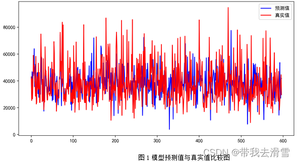
表2 模型预测效果评价指标
RMSE
MAE
0.7492
14164.27
10469.42
通过表6-2 可以看到,使用支持向量回归(SVR)预测y(每平方米价格),其预测效果较好,达到了0.7492。
(2)预测 y1(房屋总价)
支持向量回归(SVR)的部分预测结果见表3,模型预测值与真实值的比较见图2,模型的评价指标见表4,代码见附件。
表3 SVR部分预测结果表
真实值
预测值
真实值
预测值
真实值
预测值
230
246
193
183
570
486
350
392
235
257
215
251
175
224
230
292
730
799
750
752
325
366
225
256
769
554
235
248
195
219
508
503
280
301
480
445
880
990
440
357
600
530
258
279
458
238
320
324
460
542
510
471
380
450
328
598
250
150
530
354
315
214
280
286
158
23
200
323
580
392
580
375
152
223
730
566
570
486
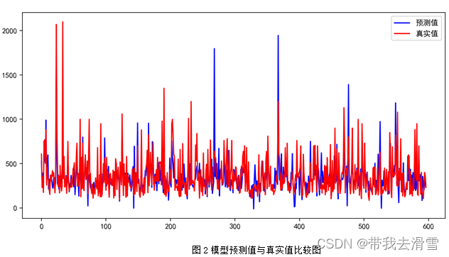
表4 模型预测效果评价指标
RMSE
MAE
0.4465
172.41
110.89
通过表4可以看到,使用支持向量回归(SVR)预测 y1 (房屋总价),其预测效果较差, 只达到了0.4465。
3、随机森林回归
3.1 基本原理
随机森林回归算法(Random Forest Regression)是随机森林(Random Forest)的重要应用分支。随机森林回归模型通过随机抽取样本和特征,建立多棵相互不关联的决策树,通过并行的方式获得预测结果。每棵决策树都能通过抽取的样本和特征得出一个预测结果,通过综合所有树的结果取平均值,得到整个森林的回归预测结果。
3.2 随机森林回归预测房价
(1)预测y(每平方米价格)
部分预测结果见表5,模型预测值与真实值的比较见图3,模型的评价指标见表6,特征变量重要性程度见图4。
表5 部分预测结果表
真实值
预测值
真实值
预测值
真实值
预测值
43066
41603
44095
48083
48572
49060
41568
44930
47538
40109
33885
33400
47038
49869
39167
43594
34039
33163
51502
53119
32800
38749
69263
47932
40630
38450
25664
33913
60798
50518
38017
35283
25782
32425
29289
47061
36527
38607
39119
30230
29771
44685
33207
35792
50567
46673
37479
33603
53158
36441
30000
38889
38937
43056
34000
34300
30975
42002
17390
33836
46280
38148
28747
38848
25376
38680
23883
34620
30590
38215
40141
33607
23870
30230
42719
47383
28667
27297
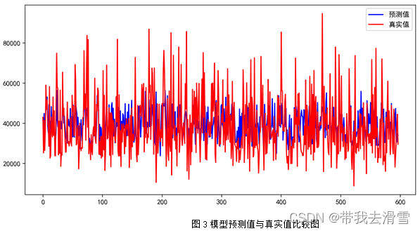
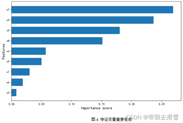
表6模型预测效果评价指标
RMSE
MAE
0.792
12502.87
9700.34
通过图4可以看到,使用随机森林回归预测y(每平方米价格),特征变量的重要程度从高到低依次是x7 (房屋附近有无地铁)、x5 (有无电梯)、x3 (房屋面积)、x8 (关注度)、x4 (房屋装修情况)、x9 (看房次数)、x1 (房屋的卧室数量)、x2 (房屋的客厅数量)。通过表6可以发现,使用随机森林回归预测y(每平方米价格),其预测效果较好, 达到了0.792。
(2)预测 y1(房屋总价)
随机森林回归部分预测结果见表7,模型预测值与真实值的比较见图5,模型的评价指标见表8。
表7 部分预测结果表
真实值
预测值
真实值
预测值
真实值
预测值
880
888
195
207
950
846
258
246
480
460
125
157
460
463
600
582
160
204
328
551
320
239
285
386
315
190
380
399
500
1371
200
394
530
465
285
324
152
204
158
176
560
882
370
398
580
409
323
269
305
324
270
263
200
227
350
363
110
154
570
331
420
293
193
168
270
323
357
393
215
296
415
368
398
327
155
196
250
589
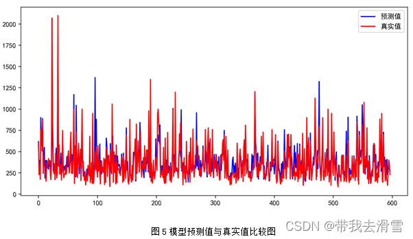
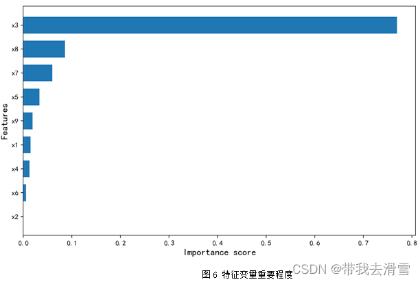
表8模型预测效果评价指标
RMSE
MAE
0.7596
12502.87
9700.33
通过图6可以看到,使用随机森林回归预测 *y*1 (房屋总价),特征变量的重要程度从高到低依次是*x*3 (房屋面积)、*x*8 (关注度)、*x*7 (房屋附近有无地铁)、*x*5 (有无电梯)、*x*9 (看房次数)、*x*1 (房屋的卧室数量)、*x*4 (房屋装修情况)、*x*6 (房屋所在楼层位置)、*x*2 (房屋的客厅数量)。通过表6-8可以发现,使用随机森林回归预测*y*1 (房屋总价),其预测效果较好,达到了0.7596。
(1)支持向量回归预测房价
import numpy as np
import pandas as pd
import matplotlib.pyplot as plt
import seaborn as sns
from sklearn import preprocessing
from sklearn.preprocessing import StandardScaler
from sklearn.svm import LinearSVR
from sklearn.svm import SVR
from sklearn.ensemble import RandomForestRegressor
from sklearn.model_selection import train_test_split
from sklearn.metrics import mean_squared_error
from sklearn.metrics import mean_absolute_error
from sklearn.metrics import r2_score
get_ipython().run_line_magic('matplotlib', 'inline')
plt.rcParams['font.sans-serif'] = ['SimHei']
plt.rcParams['axes.unicode_minus'] = False
from IPython.core.interactiveshell import InteractiveShell
InteractiveShell.ast_node_interactivity = 'all'
import warnings
warnings.filterwarnings("ignore")
# 数据集划分与数据标准化
data = pd.read_excel(r'E:\工作\硕士\学习\统计软件python\期末作业\清洗后数据.xlsx')
data
X_train, X_valid, y_train, y_valid = train_test_split(X, y, test_size=0.2, random_state = 1234)
将数据随机划分成80%训练集和20%测试集
train, test = train_test_split(data, test_size=0.2, random_state = 1234)
train = train.reset_index(drop = True)
test = test.reset_index(drop = True)
train
test
X_train, X_test = train.iloc[:,:-2], test.iloc[:,:-2]
Y_train, Y_test = train.iloc[:,-2], test.iloc[:,-2]
Y1_train, Y1_test = train.iloc[:,-1], test.iloc[:,-1]
数据标准化(主要是为了构建支持向量机做准备)
scaler = StandardScaler()
x_scaler = scaler.fit(X_train)
x_train = x_scaler.fit_transform(X_train)
x_test = x_scaler.fit_transform(X_test)
y_scaler = scaler.fit(Y_train.values.reshape(-1,1))
y_train = y_scaler.fit_transform(Y_train.values.reshape(-1,1))
y_test = y_scaler.fit_transform(Y_test.values.reshape(-1,1))
y1_scaler = scaler.fit(Y1_train.values.reshape(-1,1))
y1_train = y1_scaler.fit_transform(Y1_train.values.reshape(-1,1))
y1_test = y1_scaler.fit_transform(Y1_test.values.reshape(-1,1))
## 支持向量机
### 对y
#### RBF_SVR
rbf_svr = SVR(kernel = "rbf", C = 100, epsilon = 0.1)
rbf_svr.fit(x_train, y_train)
预测
rbf_svr_pred = rbf_svr.predict(x_test)
y_scaler = scaler.fit(Y_train.values.reshape(-1,1))
y_scaler.fit_transform(Y_train.values.reshape(-1,1))
rbf_svr_pred = y_scaler.inverse_transform(rbf_svr_pred.reshape(-1,1))
模型评价
rbf_svr_rmse = np.sqrt(mean_squared_error(Y_test,rbf_svr_pred)) #RMSE
rbf_svr_mae = mean_absolute_error(Y_test,rbf_svr_pred) #MAE
rbf_svr_r2 = r2_score(Y_test, rbf_svr_pred) # R2
print("R^2 of RBF_SVR: ", rbf_svr_r2)
print("The RMSE of RBF_SVR: ", rbf_svr_rmse)
print("The MAE of RBF_SVR: ", rbf_svr_mae)
输出预测值和真实值矩阵
rbf_svr_pred_true = pd.concat([pd.DataFrame(rbf_svr_pred), pd.DataFrame(Y_test)], axis = 1)
rbf_svr_pred_true.columns = ['预测值', '真实值']
rbf_svr_pred_true.to_excel(r' E:\工作\硕士\学习\统计软件python\期末作业\径向基核支持向量机预测y.xlsx', index = False)
比较图
plt.subplots(figsize=(10,5), dpi = 200)
plt.plot(rbf_svr_pred, color = 'b', label = '预测值')
plt.plot(Y_test, color = 'r', label = '真实值')
plt.legend(loc = 0)
#### POLY_SVR
poly_svr = SVR(kernel="poly", degree=2, C=100, epsilon=0.1, gamma="scale")
poly_svr.fit(x_train, y_train)
预测y
poly_svr_pred = poly_svr.predict(x_test)
y_scaler = scaler.fit(Y_train.values.reshape(-1,1))
y_scaler.fit_transform(Y_train.values.reshape(-1,1))
poly_svr_pred = y_scaler.inverse_transform(poly_svr_pred.reshape(-1,1))
模型评价
poly_svr_rmse = np.sqrt(mean_squared_error(Y_test,poly_svr_pred)) #RMSE
poly_svr_mae = mean_absolute_error(Y_test,poly_svr_pred) #MAE
poly_svr_r2 = r2_score(Y_test, poly_svr_pred) # R2
print("R^2 of POLY_SVR: ", poly_svr_r2)
print("The RMSE of POLY_SVR: ", poly_svr_rmse)
print("The MAE of PLOY_SVR: ", poly_svr_mae)
plt.subplots(figsize=(10,5), dpi = 200)
plt.plot(poly_svr_pred, color = 'b', label = '预测值')
plt.plot(Y_test, color = 'r', label = '真实值')
plt.legend(loc = 0)
### 对y1
#### RBF_SVR
rbf1_svr = SVR(kernel = "rbf", C = 100, epsilon = 0.1)
rbf1_svr.fit(x_train, y1_train)
预测y1
rbf1_svr_pred = rbf1_svr.predict(x_test)
y1_scaler = scaler.fit(Y1_train.values.reshape(-1,1))
y1_train = y1_scaler.fit_transform(Y1_train.values.reshape(-1,1))
rbf1_svr_pred = y1_scaler.inverse_transform(rbf1_svr_pred.reshape(-1,1))
模型评价
rbf1_svr_rmse = np.sqrt(mean_squared_error(Y1_test,rbf1_svr_pred)) #RMSE
rbf1_svr_mae = mean_absolute_error(Y1_test,rbf1_svr_pred) #MAE
rbf1_svr_r2 = r2_score(Y1_test, rbf1_svr_pred) # R2
print("R^2 of RBF_SVR: ", rbf1_svr_r2)
print("The RMSE of RBF_SVR: ", rbf1_svr_rmse)
print("The MAE of RBF_SVR: ", rbf1_svr_mae)
输出预测值和真实值矩阵
rbf1_svr_pred_true = pd.concat([pd.DataFrame(rbf1_svr_pred), pd.DataFrame(Y1_test)], axis = 1)
rbf1_svr_pred_true.columns = ['预测值', '真实值']
rbf1_svr_pred_true.to_excel(r' E:\工作\硕士\学习\统计软件python\期末作业\径向基核支持向量机预测y1.xlsx', index = False)
画图
plt.subplots(figsize=(10,5), dpi = 200)
plt.plot(rbf1_svr_pred, color = 'b', label = '预测值')
plt.plot(Y1_test, color = 'r', label = '真实值')
plt.legend(loc = 0)
#### POLY_SVR
poly1_svr = SVR(kernel="poly", degree=3, C=100, epsilon=0.1, gamma="scale")
poly1_svr.fit(x_train, y1_train)
预测
poly1_svr_pred = poly1_svr.predict(x_test)
y1_scaler = scaler.fit(Y1_train.values.reshape(-1,1))
y1_train = y1_scaler.fit_transform(Y1_train.values.reshape(-1,1))
poly1_svr_pred = y1_scaler.inverse_transform(poly1_svr_pred.reshape(-1,1))
模型评价
poly1_svr_rmse = np.sqrt(mean_squared_error(Y1_test,poly1_svr_pred)) #RMSE
poly1_svr_mae = mean_absolute_error(Y1_test,poly1_svr_pred) #MAE
poly1_svr_r2 = r2_score(Y1_test, poly1_svr_pred) # R2
print("R^2 of POLY_SVR: ", poly1_svr_r2)
print("The RMSE of POLY_SVR: ", poly1_svr_rmse)
print("The MAE of POLY_SVR: ", poly1_svr_mae)
plt.subplots(figsize=(10,5), dpi = 200)
plt.plot(poly1_svr_pred, color = 'b', label = '预测值')
plt.plot(Y1_test, color = 'r', label = '真实值')
plt.legend(loc = 0)
(2)随机森林回归预测房价
模型建立与预测
随机森林
对y
rf = RandomForestRegressor(n_estimators = 1000, max_depth = 6, random_state = 1234)
rf.fit(X_train, Y_train)
rf_pred = rf.predict(X_test)
模型评价
rf_rmse = np.sqrt(mean_squared_error(Y_test,rf_pred)) #RMSE
rf_mae = mean_absolute_error(Y_test,rf_pred) #MAE
rf_r2 = r2_score(Y_test, rf_pred) # R2
print("R^2 of RandomForest: ", rf_r2)
print("The RMSE of RandomForest: ", rf_rmse)
print("The MAE of RandomForest: ", rf_mae)
输出预测值和真实值矩阵
rf_pred_true = pd.concat([pd.DataFrame(rf_pred), pd.DataFrame(Y_test)], axis = 1)
rf_pred_true.columns = ['预测值', '真实值']
rf_pred_true.to_excel(r'E:\工作\硕士\学习\统计软件python\期末作业\ \随机森林预测y.xlsx ', index = False)
比较图
plt.subplots(figsize=(10,5), dpi = 200)
plt.plot(rf_pred, color = 'b', label = '预测值')
plt.plot(Y_test, color = 'r', label = '真实值')
plt.legend(loc = 0)
dic = dict(zip(X_train.columns, rf.feature_importances_))
dic = dict(sorted(dic.items(),key=lambda x:x[1]))
rf_fea_name = [key for key,value in dic.items() ]
rf_fea = [value for key,value in dic.items() ]
plt.figure(figsize = (10,6), dpi = 200)
plt.barh(rf_fea_name, rf_fea, height = 0.7)
plt.xlabel('Importance score', fontsize = 13)
plt.ylabel('Features', fontsize = 13)
### 对y1
rf1 = RandomForestRegressor(n_estimators = 1000, max_depth = 6, random_state = 1234)
rf1.fit(X_train, Y1_train)
rf1_pred = rf1.predict(X_test)
模型评价
rf1_rmse = np.sqrt(mean_squared_error(Y1_test,rf1_pred)) #RMSE
rf1_mae = mean_absolute_error(Y1_test,rf1_pred) #MAE
rf1_r2 = r2_score(Y1_test, rf1_pred) # R2
print("R^2 of RandomForest: ", rf1_r2)
print("The RMSE of RandomForest: ", rf1_rmse)
print("The MAE of RandomForest: ", rf1_mae)
输出预测值和真实值矩阵
rf1_pred_true = pd.concat([pd.DataFrame(rf1_pred), pd.DataFrame(Y1_test)], axis = 1)
rf1_pred_true.columns = ['预测值', '真实值']
rf1_pred_true.to_excel(r' E:\工作\硕士\学习\统计软件python\期末作业\随机森林预测y1', index = False)
比较图
plt.subplots(figsize=(10,5), dpi = 200)
plt.plot(rf1_pred, color = 'b', label = '预测值')
plt.plot(Y1_test, color = 'r', label = '真实值')
plt.legend(loc = 0)
dic = dict(zip(X_train.columns, rf1.feature_importances_))
dic = dict(sorted(dic.items(),key=lambda x:x[1]))
rf_fea_name = [key for key,value in dic.items() ]
rf_fea = [value for key,value in dic.items() ]
plt.figure(figsize = (10,6), dpi = 200)
plt.barh(rf_fea_name, rf_fea, height = 0.7)
plt.xlabel('Importance score', fontsize = 13)
plt.ylabel('Features', fontsize = 13)
需要数据集的家人们可以去百度网盘(永久有效)获取:
链接:https://pan.baidu.com/s/16GeXC9_f6KI4lS2wQ-Z1VQ?pwd=2138
提取码:2138
更多优质内容持续发布中,请移步主页
点赞+关注,下次不迷路!
版权归原作者 带我去滑雪 所有, 如有侵权,请联系我们删除。