人脸识别经典网络-MTCNN（含Python源码实现）

人脸检测-mtcnn

本文参加新星计划人工智能赛道：https://bbs.csdn.net/topics/613989052

文章目录

1. 人脸检测

1.1 人脸检测概述

人脸检测或者识别，都是根据人的脸部特征信息进行身份识别的一种生物识别术。用摄像机或摄像头采集含有人脸的图像或视频流，并自动在图像中检测和跟踪人脸，进而对检测到的人脸进行脸部识别的一系列相关技术，通常也叫做人像识别、面部识别。

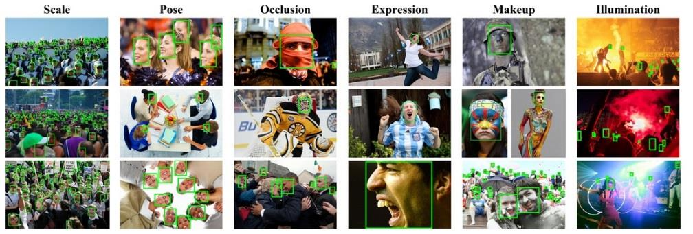
1.2 人脸检测的难点

人脸识别被认为是生物特征识别领域甚至人工智能领域最困难的研究课题之一。人脸识别的难点是由于人脸作为生物特征的特点而导致的，难点主要包括以下部分：

• 相似性：从人脸的构造上来看，个体之间的人脸构造区别不大，甚至人脸器官的构造都很相似。这种相似性对于利用人脸进行定位是能偶提供很大的便利的，但同时对于个体的区分确实难的。
• 易变性：抛去构造仅仅关注外形的话，人脸的外形又是十分多变的，面部表情多变，而在不同观察角度，人脸的视觉图像也相差很大，另外，人脸识别还受光照条件（例如白天和夜晚，室内和室外等）、人脸的很多遮盖物（例如口罩、墨镜、头发、胡须等）、年龄等多方面因素的影响。

在人脸识别中，第一类的变化是应该放大而作为区分个体的标准的，而第二类的变化应该消除，因为它们可以代表同一个个体。通常称第一类变化为类间变化（inter-class difference），而称第二类变化为类内变化（intra-class difference）。对于人脸，类内变化往往大于类间变化，从而使在受类内变化干扰的情况下利用类间变化区分个体变得异常困难。

1.3 人脸检测的应用场景

人脸识别主要用于身份识别。
由于视频监控正在快速普及，众多的视频监控应用迫切需要一种远距离、用户非配合状态下的快速身份识别技术，以求远距离快速确认人员身份，实现智能预警。人脸识别技术无疑是最佳的选择，采用快速人脸检测技术可以从监控视频图象中实时查找人脸，并与人脸数据库进行实时比对，从而实现快速身份识别。
人脸识别产品已广泛应用于金融、司法、军队、公安、边检、政府、航天、电力、工厂、教育、医疗及众多企事业单位等领域。随着技术的进一步成熟和社会认同度的提高，人脸识别技术将应用在更多的领域。
1、企业、住宅安全和管理。如人脸识别门禁考勤系统，人脸识别防盗门等。
2、电子护照及身份证。
3、公安、司法和刑侦。如利用人脸识别系统和网络，在全国范围内搜捕逃犯。
4、自助服务。
5、信息安全。如手机、计算机登录、电子政务和电子商务。

2. mtcnn

2.1 mtcnn概述

MTCNN，英文全称是Multi-task convolutional neural network，中文全称是多任务卷积神经网络，该神经网络将人脸区域检测与人脸关键点检测放在了一起。
从工程实践上，MTCNN是一种检测速度和准确率都很不错的算法，算法的推断流程有一定的启示作用。

2.2 mtcnn的网络结构

mtcnn从整体上划分分为P-Net、R-Net、和O-Net三层网络结构。各层的作用直观上感受如下图所示：

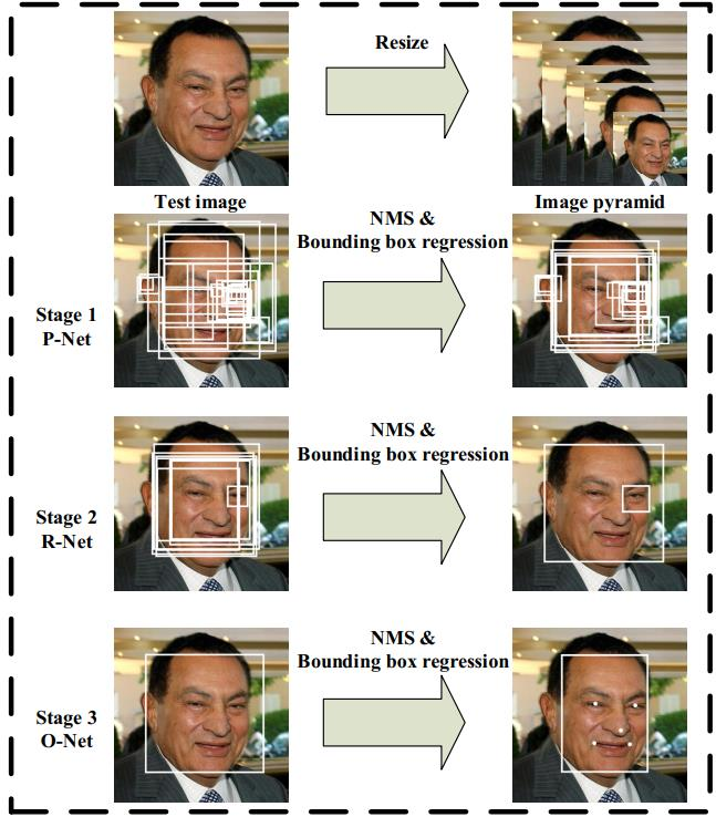
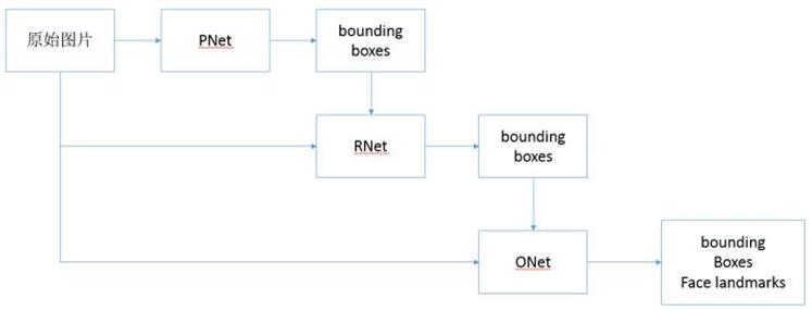
一次mtcnn对于局部信息的运作流程如下描述：

1. 由原始图片和PNet生成预测的bounding boxes。
2. 输入原始图片和PNet生成的bounding box，通过RNet，生成校正后的bounding box。
3. 输入原始图片和RNet生成的bounding box，通过ONet，生成校正后的bounding box和人脸面部轮廓关键点。

当整个图片的局部信息都进行处理之后，就能得到所有的局部人脸信息，或有或无，进行校正处理后就可以得到最后的结果。

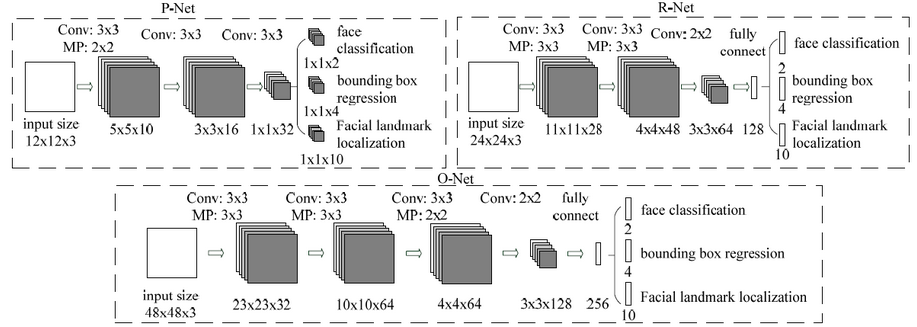
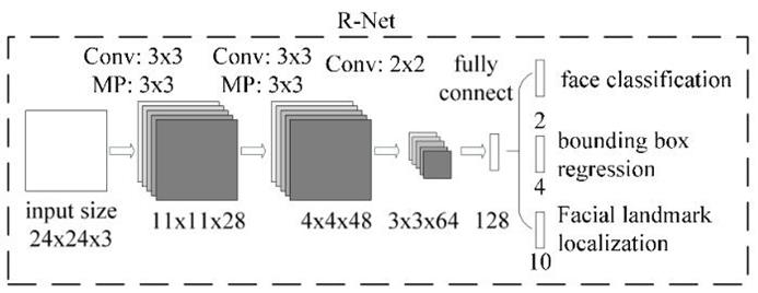
P-Net、R-Net、O-Net的网络结构如下图所示：

分析：

MTCNN主要包括三层网络，

1. 第一层P-Net将经过卷积，池化操作后输出分类（对应像素点是否存在人脸）和回归（回归box)结果。
2. 第二层网络将第一层输出的结果使用非极大抑制（NMS）来去除高度重合的候选框，并将这些候选框放入R-Net中进行精细的操作，拒绝大量错误框，再对回归框做校正，并使用NMS去除重合框，输出分支同样两个分类和回归。
3. 最后将R-Net输出认为是人脸的候选框输入到O-Net中再一次进行精细操作，拒绝掉错误的框，此时输出分支包含三个分类： a. 是否有人脸：2个输出； b. 回归：回归得到的框的起始点（或中心点）的xy坐标和框的长宽，4个输出； c. 人脸特征点定位：5个人脸特征点的xy坐标，10个输出。

三段网络都有NMS，但是所设阈值不同。

2.3 图像金字塔

mtcnn的输入尺度是任意大小的，那么输入是如何处理的呢？

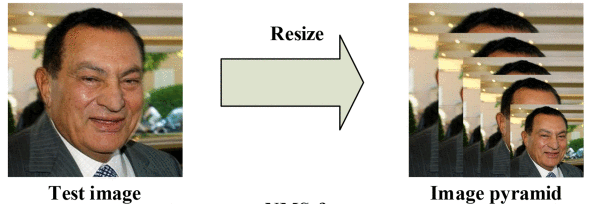
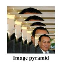
首先对图片进行Resize操作，将原始图像缩放成不同的尺度，生成图像金字塔。然后将不同尺度的图像送入到这三个子网络中进行训练，目的是为了可以检测到不同大小的人脸，从而实现多尺度目标检测。
构建方式是通过不同的缩放系数factor分别对图片的h和w进行缩放，每次缩小为原来的factor大小。

缩小后的长宽最小不可以小于12。

图片中的人脸的尺度有大有小，让识别算法不被目标尺度影响一直是个挑战。

MTCNN使用了图像金字塔来解决目标多尺度问题，即把原图按照一定的比例(如0.709)，多次等比缩放得到多尺度的图片，很像个金字塔。

为什么这里的缩放因子是0.709，因为缩放的时候若宽高都缩放

      1
     
     
      2
     
    
   
   
    \frac{1}{2}
   
  
 21​，那么缩放后的面积就变为了原本面积的
 
  
   
    
     
      1
     
     
      4
     
    
   
   
    \frac{1}{4}
   
  
 41​，如果考虑总面积缩放为原本的
 
  
   
    
     
      1
     
     
      2
     
    
   
   
    \frac{1}{2}
   
  
 21​，那么就取
 
  
   
    
     
      
       2
      
     
     
      2
     
    
    
     ≈
    
    
     0.709
    
   
   
    \frac{\sqrt{2}}{2}\approx 0.709
   
  
 22​​≈0.709，这样就达到了将总面积缩放为原本的
 
  
   
    
     
      1
     
     
      2
     
    
   
   
    \frac{1}{2}
   
  
 21​的目的。

P-NET的模型是用单尺度(12*12)的图片训练出来的。推理的时候，缩小后的长宽最小不可以小于12。
对多个尺度的输入图像做训练，训练是非常耗时的。因此通常只在推理阶段使用图像金字塔，提高算法的精度。

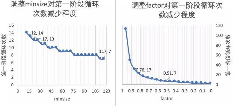
图像金字塔是有生成标准的，每次缩放的程度（factor）以及最小的兜底标准（minsize）都是需要合适的设置的，那么能够优化计算效率的合适的最小人脸尺寸（minsize）和缩放因子（factor）具有什么样的依据？

• 第一阶段会多次缩放原图得到图片金字塔，目的是为了让缩放后图片中的人脸与P-NET训练时候的图片尺度( 12 p x × 12 p x 12px\times 12px 12px×12px)接近。
• 引申优化项：先把图像缩放到一定大小，再通过factor对这个大小进行缩放。可以减少计算量。

minsize的单位为px

例：输入图片为

    1200
   
   
    p
   
   
    x
   
   
    ×
   
   
    1200
   
   
    p
   
   
    x
   
  
  
   1200px\times 1200px
  
 
1200px×1200px，设置缩放后的尺寸接近训练图片的尺度(
 
  
   
    12
   
   
    p
   
   
    x
   
   
    ×
   
   
    12
   
   
    p
   
   
    x
   
  
  
   12px\times 12px
  
 
12px×12px)

图像金字塔也有其局限性

• 生成图像金字塔的过程比较慢。
• 每种尺度的图片都需要输入进模型，相当于执行了多次的模型推理流程。

2.4 P-Net

P-Net（Proposal Network）的网络结构

网络的输入为预处理中得到的图像金字塔，P-Net中设计了一个全卷积网络（FCN）对输入的图像金字塔进行特征提取和边框回归。

全卷积神经网络没有FC全连接层，这就突破了输入维度的限制，那么其接受的输入尺寸是任意的。

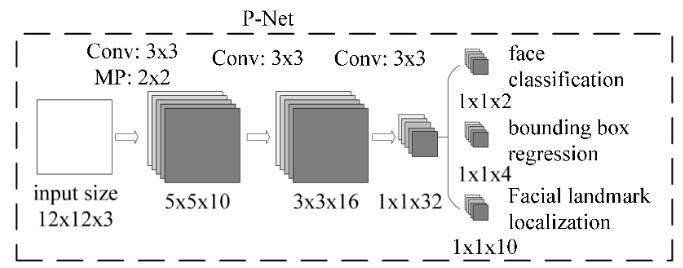
在P-Net中，经过了三次卷积和一次池化（MP：Max Pooling），输入

    12
   
   
    ×
   
   
    12
   
   
    ×
   
   
    3
   
  
  
   12\times 12 \times 3
  
 
12×12×3的尺寸变为了
 
  
   
    1
   
   
    ×
   
   
    1
   
   
    ×
   
   
    32
   
  
  
   1\times 1\times 32
  
 
1×1×32，
 
  
   
    1
   
   
    ×
   
   
    1
   
   
    ×
   
   
    32
   
  
  
   1\times 1\times 32
  
 
1×1×32的向量通过卷积得到了
 
  
   
    1
   
   
    ×
   
   
    1
   
   
    ×
   
   
    2
   
  
  
   1\times 1\times 2
  
 
1×1×2到了人脸的分类结果，相当于图像中的每个
 
  
   
    12
   
   
    ×
   
   
    12
   
  
  
   12\times 12
  
 
12×12的区域都会判断一下是否存在人脸，通道数为2，即得到两个值；第二个部分得到（bounding box regrssion）边框回归的结果，因为
 
  
   
    12
   
   
    ×
   
   
    12
   
  
  
   12\times 12
  
 
12×12的图像并不能保证，方形框能够完美的框住人脸，所以输出包含的信息都是误差信息，通道数为4，有4个方面的信息，边框左上角的横坐标的相对偏移信息、边框左上角纵坐标的相对偏移信息、标定框宽度的误差、标定框高度的误差；第三个部分给出了人脸的5个关键点的位置，分别是左眼位置、右眼位置、鼻子位置、嘴巴左位置、嘴巴右位置，每个关键位置使用两个维度表示，故而输出是
 
  
   
    1
   
   
    ×
   
   
    1
   
   
    ×
   
   
    10
   
  
  
   1\times 1\times 10
  
 
1×1×10。

P-Net应用举例

一张

    70
   
   
    ×
   
   
    70
   
  
  
   70\times 70
  
 
70×70的图，经过P网络全卷积后，输出为
 
  
   
    
     
      70
     
     
      −
     
     
      2
     
    
    
     2
    
   
   
    −
   
   
    2
   
   
    −
   
   
    2
   
   
    =
   
   
    30
   
  
  
   \frac{70-2}{2} -2 -2 =30
  
 
270−2​−2−2=30，即一个5通道的
 
  
   
    30
   
   
    ×
   
   
    30
   
  
  
   30\times 30
  
 
30×30的特征图。这就意味着该图经过p的一次滑窗操作，得到
 
  
   
    30
   
   
    ×
   
   
    30
   
   
    =
   
   
    900
   
  
  
   30\times 30=900
  
 
30×30=900个建议框，而每个建议框对应1个置信度与4个偏移量。再经nms把置信度分数大于设定的阈值0.6对应的建议框保留下来，将其对应的边框偏移量经边框回归操作，得到在原图中的坐标信息，即得到符合P-Net的这些建议框了。之后传给R-Net。

2.5 R-Net

R-Net（Refine Network），从网络图可以看到，该网络结构只是和P-Net网络结构多了一个全连接层。图片在输入R-Net之前，都需要缩放到24x24x3。网络的输出与P-Net是相同的，R-Net的目的是为了去除大量的非人脸框。

2.6 O-Net

O-Net（Output Network），该层比R-Net层又多了一层卷积层，所以处理的结果会更加精细。输入的图像大小48x48x3，输出包括N个边界框的坐标信息，score以及关键点位置。

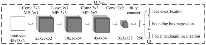
从P-Net到R-Net，再到最后的O-Net，网络输入的图像越来越大，卷积层的通道数越来越多，网络的深度（层数）也越来越深，因此识别人脸的准确率应该也是越来越高的。

3. 工程实践（基于Keras）

点击此处下载人脸数据集。该数据集有32,203张图片，共有93,703张脸被标记。

MTCNN网络定义，按照上述网络结构完成定义，代码按照P-Net、R-Net、O-Net进行模块化设计，在mtcnn的网络构建过程中将其整合。mtcnn.py代码如下：

from keras.layers import Conv2D, Input,MaxPool2D, Reshape,Activation,Flatten, Dense, Permute
from keras.layers.advanced_activations import PReLU
from keras.models import Model, Sequential
import tensorflow as tf
import numpy as np
import utils
import cv2
#-----------------------------##   粗略获取人脸框#   输出bbox位置和是否有人脸#-----------------------------#defcreate_Pnet(weight_path):input= Input(shape=[None,None,3])
    x = Conv2D(10,(3,3), strides=1, padding='valid', name='conv1')(input)
    x = PReLU(shared_axes=[1,2],name='PReLU1')(x)
    x = MaxPool2D(pool_size=2)(x)
    x = Conv2D(16,(3,3), strides=1, padding='valid', name='conv2')(x)
    x = PReLU(shared_axes=[1,2],name='PReLU2')(x)
    x = Conv2D(32,(3,3), strides=1, padding='valid', name='conv3')(x)
    x = PReLU(shared_axes=[1,2],name='PReLU3')(x)
    classifier = Conv2D(2,(1,1), activation='softmax', name='conv4-1')(x)# 无激活函数，线性。
    bbox_regress = Conv2D(4,(1,1), name='conv4-2')(x)
    model = Model([input],[classifier, bbox_regress])
    model.load_weights(weight_path, by_name=True)return model
#-----------------------------##   mtcnn的第二段#   精修框#-----------------------------#defcreate_Rnet(weight_path):input= Input(shape=[24,24,3])# 24,24,3 -> 11,11,28
    x = Conv2D(28,(3,3), strides=1, padding='valid', name='conv1')(input)
    x = PReLU(shared_axes=[1,2], name='prelu1')(x)
    x = MaxPool2D(pool_size=3,strides=2, padding='same')(x)# 11,11,28 -> 4,4,48
    x = Conv2D(48,(3,3), strides=1, padding='valid', name='conv2')(x)
    x = PReLU(shared_axes=[1,2], name='prelu2')(x)
    x = MaxPool2D(pool_size=3, strides=2)(x)# 4,4,48 -> 3,3,64
    x = Conv2D(64,(2,2), strides=1, padding='valid', name='conv3')(x)
    x = PReLU(shared_axes=[1,2], name='prelu3')(x)# 3,3,64 -> 64,3,3
    x = Permute((3,2,1))(x)
    x = Flatten()(x)# 576 -> 128
    x = Dense(128, name='conv4')(x)
    x = PReLU( name='prelu4')(x)# 128 -> 2 128 -> 4
    classifier = Dense(2, activation='softmax', name='conv5-1')(x)
    bbox_regress = Dense(4, name='conv5-2')(x)
    model = Model([input],[classifier, bbox_regress])
    model.load_weights(weight_path, by_name=True)return model
#-----------------------------##   mtcnn的第三段#   精修框并获得五个点#-----------------------------#defcreate_Onet(weight_path):input= Input(shape =[48,48,3])# 48,48,3 -> 23,23,32
    x = Conv2D(32,(3,3), strides=1, padding='valid', name='conv1')(input)
    x = PReLU(shared_axes=[1,2],name='prelu1')(x)
    x = MaxPool2D(pool_size=3, strides=2, padding='same')(x)# 23,23,32 -> 10,10,64
    x = Conv2D(64,(3,3), strides=1, padding='valid', name='conv2')(x)
    x = PReLU(shared_axes=[1,2],name='prelu2')(x)
    x = MaxPool2D(pool_size=3, strides=2)(x)# 8,8,64 -> 4,4,64
    x = Conv2D(64,(3,3), strides=1, padding='valid', name='conv3')(x)
    x = PReLU(shared_axes=[1,2],name='prelu3')(x)
    x = MaxPool2D(pool_size=2)(x)# 4,4,64 -> 3,3,128
    x = Conv2D(128,(2,2), strides=1, padding='valid', name='conv4')(x)
    x = PReLU(shared_axes=[1,2],name='prelu4')(x)# 3,3,128 -> 128,12,12
    x = Permute((3,2,1))(x)# 1152 -> 256
    x = Flatten()(x)
    x = Dense(256, name='conv5')(x)
    x = PReLU(name='prelu5')(x)# 鉴别# 256 -> 2 256 -> 4 256 -> 10 
    classifier = Dense(2, activation='softmax',name='conv6-1')(x)
    bbox_regress = Dense(4,name='conv6-2')(x)
    landmark_regress = Dense(10,name='conv6-3')(x)
    model = Model([input],[classifier, bbox_regress, landmark_regress])
    model.load_weights(weight_path, by_name=True)return model
classmtcnn():def__init__(self):
        self.Pnet = create_Pnet('model_data/pnet.h5')
        self.Rnet = create_Rnet('model_data/rnet.h5')
        self.Onet = create_Onet('model_data/onet.h5')defdetectFace(self, img, threshold):#-----------------------------##   归一化，加快收敛速度#   把[0,255]映射到(-1,1)#-----------------------------#
        copy_img =(img.copy()-127.5)/127.5
        origin_h, origin_w, _ = copy_img.shape
        #-----------------------------##   计算原始输入图像#   每一次缩放的比例#-----------------------------#
        scales = utils.calculateScales(img)
        out =[]#-----------------------------##   粗略计算人脸框#   pnet部分#-----------------------------#for scale in scales:
            hs =int(origin_h * scale)
            ws =int(origin_w * scale)
            scale_img = cv2.resize(copy_img,(ws, hs))
            inputs = scale_img.reshape(1,*scale_img.shape)# 图像金字塔中的每张图片分别传入Pnet得到output
            output = self.Pnet.predict(inputs)# 将所有output加入out
            out.append(output)
        image_num =len(scales)
        rectangles =[]for i inrange(image_num):# 有人脸的概率
            cls_prob = out[i][0][0][:,:,1]# 其对应的框的位置
            roi = out[i][1][0]# 取出每个缩放后图片的长宽
            out_h, out_w = cls_prob.shape
            out_side =max(out_h, out_w)print(cls_prob.shape)# 解码过程
            rectangle = utils.detect_face_12net(cls_prob, roi, out_side,1/ scales[i], origin_w, origin_h, threshold[0])
            rectangles.extend(rectangle)# 进行非极大抑制
        rectangles = utils.NMS(rectangles,0.7)iflen(rectangles)==0:return rectangles
        #-----------------------------##   稍微精确计算人脸框#   Rnet部分#-----------------------------#
        predict_24_batch =[]for rectangle in rectangles:
            crop_img = copy_img[int(rectangle[1]):int(rectangle[3]),int(rectangle[0]):int(rectangle[2])]
            scale_img = cv2.resize(crop_img,(24,24))
            predict_24_batch.append(scale_img)
        predict_24_batch = np.array(predict_24_batch)
        out = self.Rnet.predict(predict_24_batch)
        cls_prob = out[0]
        cls_prob = np.array(cls_prob)
        roi_prob = out[1]
        roi_prob = np.array(roi_prob)
        rectangles = utils.filter_face_24net(cls_prob, roi_prob, rectangles, origin_w, origin_h, threshold[1])iflen(rectangles)==0:return rectangles
        #-----------------------------##   计算人脸框#   onet部分#-----------------------------#
        predict_batch =[]for rectangle in rectangles:
            crop_img = copy_img[int(rectangle[1]):int(rectangle[3]),int(rectangle[0]):int(rectangle[2])]
            scale_img = cv2.resize(crop_img,(48,48))
            predict_batch.append(scale_img)
        predict_batch = np.array(predict_batch)
        output = self.Onet.predict(predict_batch)
        cls_prob = output[0]
        roi_prob = output[1]
        pts_prob = output[2]
        rectangles = utils.filter_face_48net(cls_prob, roi_prob, pts_prob, rectangles, origin_w, origin_h, threshold[2])return rectangles

当有了mtcnn定义之后，可以利用其作为自己的模块来进行调用，推理，detect.py代码如下：

import cv2
import numpy as np
from mtcnn import mtcnn
img = cv2.imread('img/test1.jpg')
model = mtcnn()
threshold =[0.5,0.6,0.7]# 三段网络的置信度阈值不同
rectangles = model.detectFace(img, threshold)
draw = img.copy()for rectangle in rectangles:if rectangle isnotNone:
        W =-int(rectangle[0])+int(rectangle[2])
        H =-int(rectangle[1])+int(rectangle[3])
        paddingH =0.01* W
        paddingW =0.02* H
        crop_img = img[int(rectangle[1]+paddingH):int(rectangle[3]-paddingH),int(rectangle[0]-paddingW):int(rectangle[2]+paddingW)]if crop_img isNone:continueif crop_img.shape[0]<0or crop_img.shape[1]<0:continue
        cv2.rectangle(draw,(int(rectangle[0]),int(rectangle[1])),(int(rectangle[2]),int(rectangle[3])),(255,0,0),1)for i inrange(5,15,2):
            cv2.circle(draw,(int(rectangle[i +0]),int(rectangle[i +1])),2,(0,255,0))
cv2.imwrite("img/out.jpg",draw)
cv2.imshow("test", draw)
c = cv2.waitKey(0)

其中，用到的工具类助手如下，实现了非极大值抑制已经网络的后处理等过程逻辑。

import sys
from operator import itemgetter
import numpy as np
import cv2
import matplotlib.pyplot as plt
#-----------------------------##   计算原始输入图像#   每一次缩放的比例#-----------------------------#defcalculateScales(img):
    copy_img = img.copy()
    pr_scale =1.0
    h,w,_ = copy_img.shape
    # 引申优化项  = resize(h*500/min(h,w), w*500/min(h,w))ifmin(w,h)>500:
        pr_scale =500.0/min(h,w)
        w =int(w*pr_scale)
        h =int(h*pr_scale)elifmax(w,h)<500:
        pr_scale =500.0/max(h,w)
        w =int(w*pr_scale)
        h =int(h*pr_scale)
    scales =[]
    factor =0.709
    factor_count =0
    minl =min(h,w)while minl >=12:
        scales.append(pr_scale*pow(factor, factor_count))
        minl *= factor
        factor_count +=1return scales
#-------------------------------------##   对pnet处理后的结果进行处理#-------------------------------------#defdetect_face_12net(cls_prob,roi,out_side,scale,width,height,threshold):
    cls_prob = np.swapaxes(cls_prob,0,1)
    roi = np.swapaxes(roi,0,2)
    stride =0# stride略等于2if out_side !=1:
        stride =float(2*out_side-1)/(out_side-1)(x,y)= np.where(cls_prob>=threshold)
    boundingbox = np.array([x,y]).T
    # 找到对应原图的位置
    bb1 = np.fix((stride *(boundingbox)+0)* scale)
    bb2 = np.fix((stride *(boundingbox)+11)* scale)# plt.scatter(bb1[:,0],bb1[:,1],linewidths=1)# plt.scatter(bb2[:,0],bb2[:,1],linewidths=1,c='r')# plt.show()
    boundingbox = np.concatenate((bb1,bb2),axis =1)
    
    dx1 = roi[0][x,y]
    dx2 = roi[1][x,y]
    dx3 = roi[2][x,y]
    dx4 = roi[3][x,y]
    score = np.array([cls_prob[x,y]]).T
    offset = np.array([dx1,dx2,dx3,dx4]).T
    boundingbox = boundingbox + offset*12.0*scale
    
    rectangles = np.concatenate((boundingbox,score),axis=1)
    rectangles = rect2square(rectangles)
    pick =[]for i inrange(len(rectangles)):
        x1 =int(max(0,rectangles[i][0]))
        y1 =int(max(0,rectangles[i][1]))
        x2 =int(min(width ,rectangles[i][2]))
        y2 =int(min(height,rectangles[i][3]))
        sc = rectangles[i][4]if x2>x1 and y2>y1:
            pick.append([x1,y1,x2,y2,sc])return NMS(pick,0.3)#-----------------------------##   将长方形调整为正方形#-----------------------------#defrect2square(rectangles):
    w = rectangles[:,2]- rectangles[:,0]
    h = rectangles[:,3]- rectangles[:,1]
    l = np.maximum(w,h).T
    rectangles[:,0]= rectangles[:,0]+ w*0.5- l*0.5
    rectangles[:,1]= rectangles[:,1]+ h*0.5- l*0.5 
    rectangles[:,2:4]= rectangles[:,0:2]+ np.repeat([l],2, axis =0).T 
    return rectangles
#-------------------------------------##   非极大抑制#-------------------------------------#defNMS(rectangles,threshold):iflen(rectangles)==0:return rectangles
    boxes = np.array(rectangles)
    x1 = boxes[:,0]
    y1 = boxes[:,1]
    x2 = boxes[:,2]
    y2 = boxes[:,3]
    s  = boxes[:,4]
    area = np.multiply(x2-x1+1, y2-y1+1)
    I = np.array(s.argsort())
    pick =[]whilelen(I)>0:
        xx1 = np.maximum(x1[I[-1]], x1[I[0:-1]])#I[-1] have hightest prob score, I[0:-1]->others
        yy1 = np.maximum(y1[I[-1]], y1[I[0:-1]])
        xx2 = np.minimum(x2[I[-1]], x2[I[0:-1]])
        yy2 = np.minimum(y2[I[-1]], y2[I[0:-1]])
        w = np.maximum(0.0, xx2 - xx1 +1)
        h = np.maximum(0.0, yy2 - yy1 +1)
        inter = w * h
        o = inter /(area[I[-1]]+ area[I[0:-1]]- inter)
        pick.append(I[-1])
        I = I[np.where(o<=threshold)[0]]
    result_rectangle = boxes[pick].tolist()return result_rectangle
#-------------------------------------##   对Rnet处理后的结果进行处理#-------------------------------------#deffilter_face_24net(cls_prob,roi,rectangles,width,height,threshold):
    
    prob = cls_prob[:,1]
    pick = np.where(prob>=threshold)
    rectangles = np.array(rectangles)
    x1  = rectangles[pick,0]
    y1  = rectangles[pick,1]
    x2  = rectangles[pick,2]
    y2  = rectangles[pick,3]
    
    sc  = np.array([prob[pick]]).T
    dx1 = roi[pick,0]
    dx2 = roi[pick,1]
    dx3 = roi[pick,2]
    dx4 = roi[pick,3]
    w   = x2-x1
    h   = y2-y1
    x1  = np.array([(x1+dx1*w)[0]]).T
    y1  = np.array([(y1+dx2*h)[0]]).T
    x2  = np.array([(x2+dx3*w)[0]]).T
    y2  = np.array([(y2+dx4*h)[0]]).T
    rectangles = np.concatenate((x1,y1,x2,y2,sc),axis=1)
    rectangles = rect2square(rectangles)
    pick =[]for i inrange(len(rectangles)):
        x1 =int(max(0,rectangles[i][0]))
        y1 =int(max(0,rectangles[i][1]))
        x2 =int(min(width ,rectangles[i][2]))
        y2 =int(min(height,rectangles[i][3]))
        sc = rectangles[i][4]if x2>x1 and y2>y1:
            pick.append([x1,y1,x2,y2,sc])return NMS(pick,0.3)#-------------------------------------##   对onet处理后的结果进行处理#-------------------------------------#deffilter_face_48net(cls_prob,roi,pts,rectangles,width,height,threshold):
    
    prob = cls_prob[:,1]
    pick = np.where(prob>=threshold)
    rectangles = np.array(rectangles)
    x1  = rectangles[pick,0]
    y1  = rectangles[pick,1]
    x2  = rectangles[pick,2]
    y2  = rectangles[pick,3]
    sc  = np.array([prob[pick]]).T
    dx1 = roi[pick,0]
    dx2 = roi[pick,1]
    dx3 = roi[pick,2]
    dx4 = roi[pick,3]
    w   = x2-x1
    h   = y2-y1
    pts0= np.array([(w*pts[pick,0]+x1)[0]]).T
    pts1= np.array([(h*pts[pick,5]+y1)[0]]).T
    pts2= np.array([(w*pts[pick,1]+x1)[0]]).T
    pts3= np.array([(h*pts[pick,6]+y1)[0]]).T
    pts4= np.array([(w*pts[pick,2]+x1)[0]]).T
    pts5= np.array([(h*pts[pick,7]+y1)[0]]).T
    pts6= np.array([(w*pts[pick,3]+x1)[0]]).T
    pts7= np.array([(h*pts[pick,8]+y1)[0]]).T
    pts8= np.array([(w*pts[pick,4]+x1)[0]]).T
    pts9= np.array([(h*pts[pick,9]+y1)[0]]).T
    x1  = np.array([(x1+dx1*w)[0]]).T
    y1  = np.array([(y1+dx2*h)[0]]).T
    x2  = np.array([(x2+dx3*w)[0]]).T
    y2  = np.array([(y2+dx4*h)[0]]).T
    rectangles=np.concatenate((x1,y1,x2,y2,sc,pts0,pts1,pts2,pts3,pts4,pts5,pts6,pts7,pts8,pts9),axis=1)
    pick =[]for i inrange(len(rectangles)):
        x1 =int(max(0,rectangles[i][0]))
        y1 =int(max(0,rectangles[i][1]))
        x2 =int(min(width ,rectangles[i][2]))
        y2 =int(min(height,rectangles[i][3]))if x2>x1 and y2>y1:
            pick.append([x1,y1,x2,y2,rectangles[i][4],
                 rectangles[i][5],rectangles[i][6],rectangles[i][7],rectangles[i][8],rectangles[i][9],rectangles[i][10],rectangles[i][11],rectangles[i][12],rectangles[i][13],rectangles[i][14]])return NMS(pick,0.3)

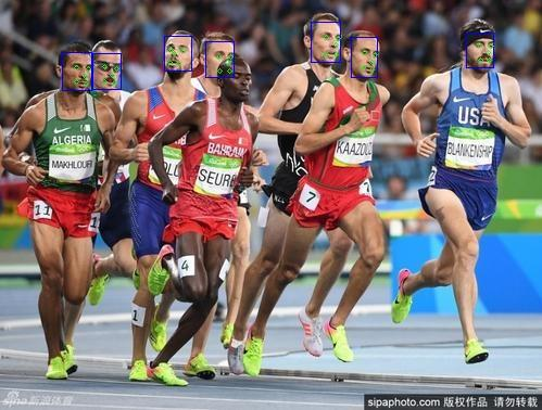
test1.jpg如下所示：

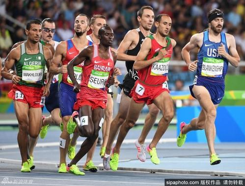
推理结果out.jpg如下所示：