
GO和KEGG富集分析
文章目录
1. 将差异表达结果的基因名称转化为id
因为GO和KEGG分析需要用到id,所以这一步需要将基因名字转换为id。具体步骤如下:
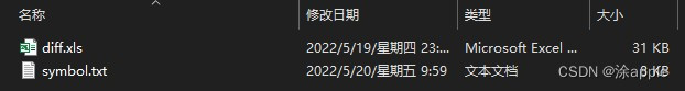
- 新建空白文件夹,将差异分析得到的diff.xls复制粘贴到文件夹中
- 因为在这里只需要diff.xls中的基因名称和logFC两列,所以只复制这两列粘贴到新建的文本文件symbol.txt,如下图所示:
- 新建R语言脚本文件symbol2id.R,代码如下:
if (!requireNamespace("BiocManager", quietly = TRUE)) install.packages("BiocManager")BiocManager::install("org.Hs.eg.db")setwd("C:\\Users\\Administrator\\Desktop\\cptac\\4_name2id") #设置工作目录library("org.Hs.eg.db") #引用包rt=read.table("symbol.txt",sep="\t",check.names=F,header=T) #读取文件genes=as.vector(rt[,1])entrezIDs <- mget(genes, org.Hs.egSYMBOL2EG, ifnotfound=NA) #找出基因对应的identrezIDs <- as.character(entrezIDs)out=cbind(rt,entrezID=entrezIDs)write.table(out,file="id.txt",sep="\t",quote=F,row.names=F) - 设置好工作目录之后,打开R软件,运行上述代码即可。运行结束在文件夹中会有id.txt,打开后如下图所示:
 可以看到后面已经有了id这一列了,至此本步骤结束。
2. GO富集分析
GO(gene ontology)是基因本体联合会(Gene Onotology Consortium)所建立的数据库,旨在建立一个适用于各种物种的、对基因和蛋白质功能进行限定和描述的、并能随着研究不断深入而更新的语言词汇标准。GO是多种生物本体语言中的一种,提供了三层结构的系统定义方式,用于描述基因产物的功能。在转录组项目中,GO功能分析一方面给出差异表达转录本的GO功能分类注释;另一方面给出差异表达转录本的GO功能显著性富集分析。
下面介绍GO分析的步骤:
- 将含有基因id的文本文件id.txt复制粘贴到新的文件夹中
- 新建R语言脚本,命名为GO.R,其代码如下:
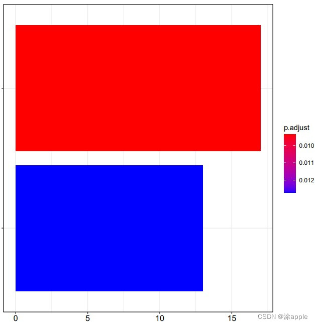
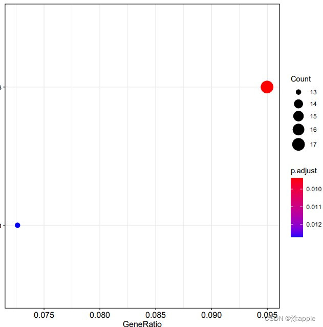
install.packages("colorspace")install.packages("stringi")install.packages("ggplot2")if (!requireNamespace("BiocManager", quietly = TRUE)) install.packages("BiocManager")BiocManager::install("DOSE")if (!requireNamespace("BiocManager", quietly = TRUE)) install.packages("BiocManager")BiocManager::install("clusterProfiler")if (!requireNamespace("BiocManager", quietly = TRUE)) install.packages("BiocManager")BiocManager::install("enrichplot")library("clusterProfiler")library("org.Hs.eg.db")library("enrichplot")library("ggplot2")setwd("C:\\Users\\Administrator\\Desktop\\cptac\\5_GO分析") #设置工作目录rt=read.table("id.txt",sep="\t",header=T,check.names=F) #读取id.txt文件rt=rt[is.na(rt[,"entrezID"])==F,] #去除基因id为NA的基因gene=rt$entrezID#GO富集分析kk <- enrichGO(gene = gene, OrgDb = org.Hs.eg.db, pvalueCutoff =0.05, qvalueCutoff = 0.05, ont="all", readable =T)write.table(kk,file="GO.txt",sep="\t",quote=F,row.names = F) #保存富集结果#柱状图pdf(file="barplot.pdf",width = 10,height = 8)barplot(kk, drop = TRUE, showCategory =10,split="ONTOLOGY") + facet_grid(ONTOLOGY~., scale='free')dev.off()#气泡图pdf(file="bubble.pdf",width = 10,height = 8)dotplot(kk,showCategory = 10,split="ONTOLOGY",orderBy = "GeneRatio") + facet_grid(ONTOLOGY~., scale='free')dev.off()这里GO分析用到的包为"clusterProfiler",画图用到的包为"enrichplot"。在代码中会设置p值和q值,设置的都是0.05,如果该条件下分析得到的可用基因较少,可将q设置为0,只看p值,但这样准确性也会降低一些。 - 打开R软件,运行上述代码,最终得到的结果如下图所示,下图按顺序分别是柱状图、气泡图以及GO分析结果。

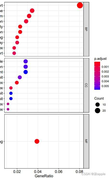
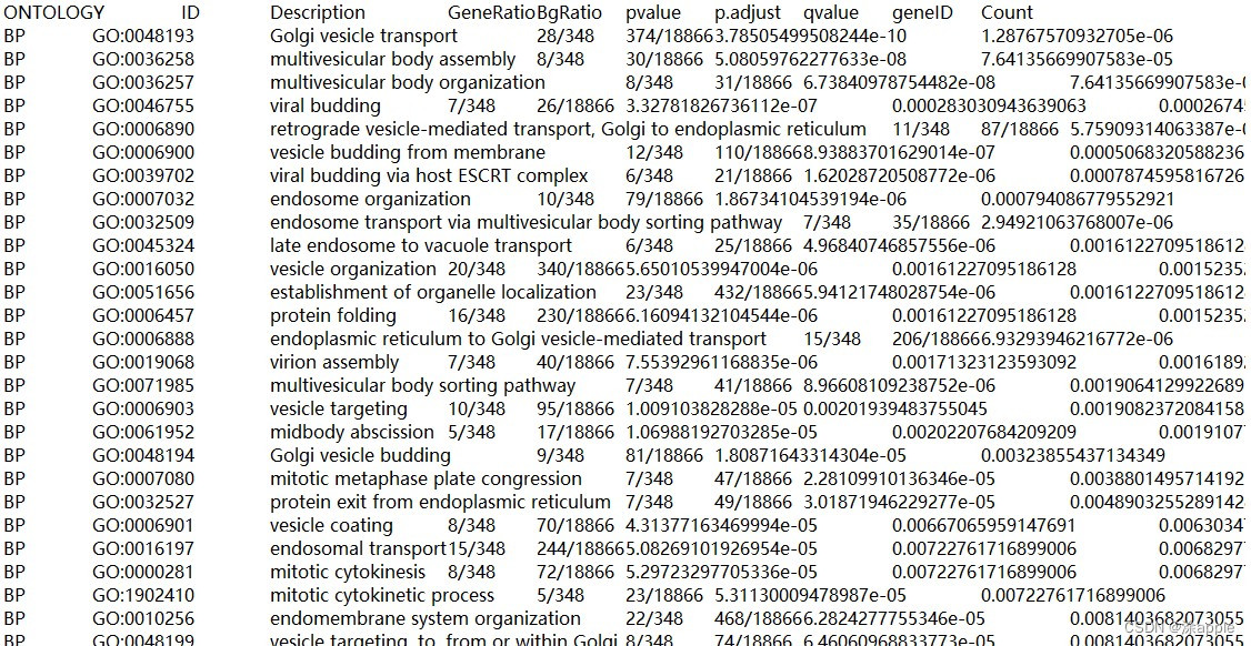
- 讲一下GO分析得到的文本文件,也就是上面三幅图中的最后一幅图,第一列是GO分析的分类,分别是BP,CC,MF;第二列是GO的id;第三列为对应的描述;第四列为基因背景的比例;第五列为p值,表示富集的显著性;第六列为p值得校正值;第七列为q值;第八列为基因id,也就是基因名称;最后一列就是富集在每个GO上的数目。对于柱状图和气泡图,会分为BP,CC,MF,每个类别颜色越红表示富集程度越高。
3. GO圈图绘制
话不多说,直接上步骤。
- 新建R语言脚本文件GOplot.R,脚本文件和GO分析得到的结果放在同一目录下,其代码如下:
install.packages("digest")install.packages("GOplot")library(GOplot)setwd("C:\\Users\\Administrator\\Desktop\\cptac\\6_GO圈图绘制") #设置工作目录ego=read.table("GO.txt", header = T,sep="\t",check.names=F) #读取kegg富集结果文件go=data.frame(Category = "All",ID = ego$ID,Term = ego$Description, Genes = gsub("/", ", ", ego$geneID), adj_pval = ego$p.adjust)#读取基因的logFC文件id.fc <- read.table("id.txt", header = T,sep="\t",check.names=F)genelist <- data.frame(ID = id.fc$gene, logFC = id.fc$logFC)row.names(genelist)=genelist[,1]circ <- circle_dat(go, genelist)termNum = 5 #限定term数目geneNum = nrow(genelist) #限定蛋白数目chord <- chord_dat(circ, genelist[1:geneNum,], go$Term[1:termNum])pdf(file="circ.pdf",width = 11,height = 10.5)GOChord(chord, space = 0.001, #基因之间的间距 gene.order = 'logFC', #按照logFC值对基因排序 gene.space = 0.25, #基因名跟圆圈的相对距离 gene.size = 4, #基因名字体大小 border.size = 0.1, #线条粗细 process.label = 7.5) #term字体大小dev.off()termCol <- c("#223D6C","#D20A13","#FFD121","#088247","#58CDD9","#7A142C","#5D90BA","#431A3D","#91612D","#6E568C","#E0367A","#D8D155","#64495D","#7CC767")pdf(file="cluster.pdf",width = 11.5,height = 9)GOCluster(circ.gsym, go$Term[1:termNum], lfc.space = 0.2, #倍数跟树间的空隙大小 lfc.width = 1, #变化倍数的圆圈宽度 term.col = termCol[1:termNum], #自定义term的颜色 term.space = 0.2, #倍数跟term间的空隙大小 term.width = 1) #富集term的圆圈宽度dev.off() - 打开R软件运行上述代码即可。最终即可得到两个圈图,如下图所示:
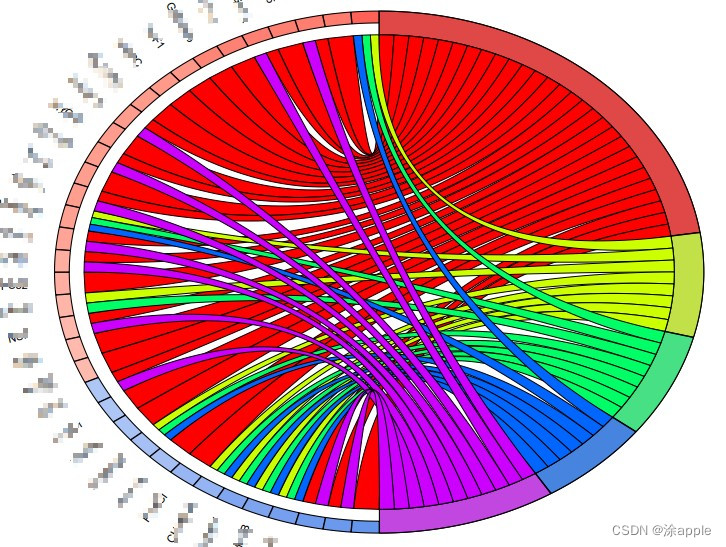 左半圆圈为基因名字,从下到上按照logFC进行排序得,圆圈右半部分为GO的名称,基因与GO之间得连线表示这个基因存在于该GO上。
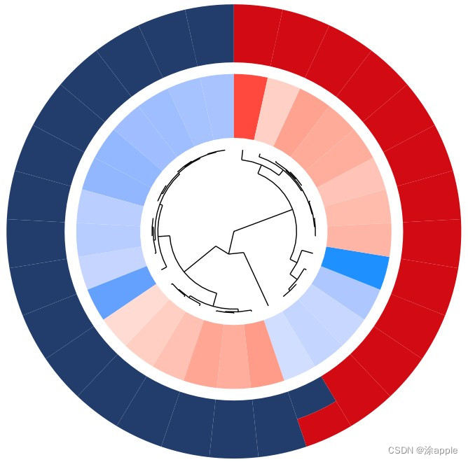
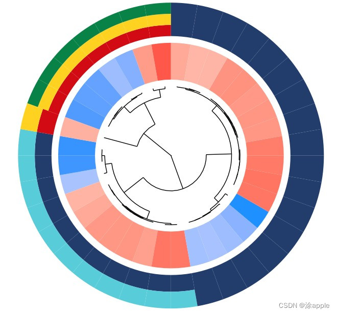 此图为聚类图,内部圆圈为基因或蛋白,颜色表示logFC的大小,内部的一个扇形表示一个基因,如果内部的一个扇形对应着外部的一个颜色的扇形,那么表示该基因只存在于这一个颜色对应的GO里面;如果内部一个扇形对应着外部三个扇形,那么表示内部的这个基因存在于三个GO里面。
4. KEGG富集分析
- 将差异分析得到的含有id的id.txt文件作为输入文件,新建文件夹,将id.txt拷贝到此文件夹下
- 新建R语言脚本文件,更改脚本文件的环境目录,代码如下:
install.packages("colorspace")install.packages("stringi")install.packages("ggplot2")if (!requireNamespace("BiocManager", quietly = TRUE)) install.packages("BiocManager")BiocManager::install("DOSE")if (!requireNamespace("BiocManager", quietly = TRUE)) install.packages("BiocManager")BiocManager::install("clusterProfiler")if (!requireNamespace("BiocManager", quietly = TRUE)) install.packages("BiocManager")BiocManager::install("enrichplot")library("clusterProfiler")library("org.Hs.eg.db")library("enrichplot")library("ggplot2")setwd("C:\\Users\\Administrator\\Desktop\\cptac\\7_KEGG分析") #设置工作目录rt=read.table("id.txt",sep="\t",header=T,check.names=F) #读取id.txt文件rt=rt[is.na(rt[,"entrezID"])==F,] #去除基因id为NA的基因gene=rt$entrezID#kegg富集分析kk <- enrichKEGG(gene = gene, organism = "hsa", pvalueCutoff =0.05, qvalueCutoff =2) #富集分析write.table(kk,file="KEGGId.txt",sep="\t",quote=F,row.names = F) #保存富集结果#柱状图pdf(file="barplot.pdf",width = 10,height = 7)barplot(kk, drop = TRUE, showCategory = 30)dev.off()#气泡图pdf(file="bubble.pdf",width = 10,height = 7)dotplot(kk, showCategory = 30,orderBy = "GeneRatio")dev.off() - 打开R软件运行上述代码,即可得到结果。
 KEGG因为数据库更新比较慢,而且分析时需要联网,因此富集到结果就会比较少。
 - 运行完之后还会得到KEGGId.txt,里面的需要将里面的id转化为基因名字。因此新建perl脚本文件,代码太长,这里就不展示了。在该文件夹目录下打开powershell窗口,输入命令perl id2symbol.pl,运行完毕之后文件夹目录下就会产生新的含有基因名字的kegg文件,文件名为kegg.txt
- 至此,KEGG分析完毕
5. KEGG圈图绘制
这里的圈图绘制和上面的GO圈图绘制步骤一样的。话不多说,直接上代码:
install.packages("digest")
install.packages("GOplot")

library(GOplot)
setwd("C:\\Users\\Administrator\\Desktop\\cptac\\8_KEGG圈图绘制")              #设置工作目录

ego=read.table("kegg.txt", header = T,sep="\t",check.names=F)       #读取kegg富集结果文件
go=data.frame(Category = "All",ID = ego$ID,Term = ego$Description, Genes = gsub("/", ", ", ego$geneID), adj_pval = ego$p.adjust)

#读取基因的logFC文件
id.fc <- read.table("id.txt", header = T,sep="\t",check.names=F)
genelist <- data.frame(ID = id.fc$gene, logFC = id.fc$logFC)
row.names(genelist)=genelist[,1]

circ <- circle_dat(go, genelist)
termNum = 2                                     #限定term数目
geneNum = nrow(genelist)                        #限定基因数目

chord <- chord_dat(circ, genelist[1:geneNum,], go$Term[1:termNum])
pdf(file="circ.pdf",width = 10,height = 9.6)
GOChord(chord,
        space = 0.001,           #基因之间的间距
        gene.order = 'logFC',    #按照logFC值对基因排序
        gene.space = 0.25,       #基因名跟圆圈的相对距离
        gene.size = 4,           #基因名字体大小
        border.size = 0.1,       #线条粗细
        process.label = 7.5)     #term字体大小
dev.off()

termCol <- c("#223D6C","#D20A13","#FFD121","#088247","#58CDD9","#7A142C","#5D90BA","#431A3D","#91612D","#6E568C","#E0367A","#D8D155","#64495D","#7CC767")
pdf(file="cluster.pdf",width = 10,height = 9.6)
GOCluster(circ.gsym,
          go$Term[1:termNum],
          lfc.space = 0.2,                   #倍数跟树间的空隙大小
          lfc.width = 1,                     #变化倍数的圆圈宽度
          term.col = termCol[1:termNum],     #自定义term的颜色
          term.space = 0.2,                  #倍数跟term间的空隙大小
          term.width = 1)                    #富集term的圆圈宽度
dev.off()
这里将代码的工作环境更改一下,然后将kegg分析所得到的kegg.txt和之前的id.txt复制到同一目录下,然后打开R软件运行代码即可。得到的圈图如下: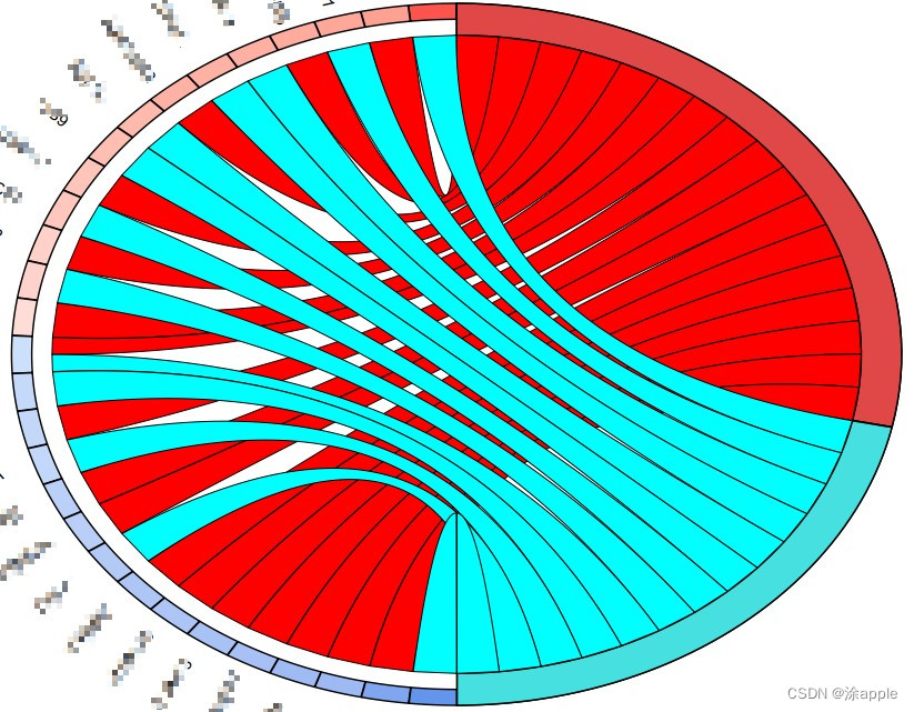
至此,KEGG圈图绘制结束。
本文转载自: https://blog.csdn.net/tqptr_opqww/article/details/124881210
版权归原作者 涂apple 所有, 如有侵权,请联系我们删除。
版权归原作者 涂apple 所有, 如有侵权,请联系我们删除。