YOLO v5 代码精读（1） detect模块以及非极大值抑制

目录

YOLO简介

YOLO 是目前最先进的目标检测模型之一，现在博客上常有的是如何使用YOLO模型训练自己的数据集，而鲜有对YOLO代码的精读。我认为只有对算法和代码实现有全面的了解，才能将YOLO使用的更加得心应手。

这里的代码精读为YOLO v5，github版本为6.0。版本不同代码也会有所不同，请结合源码阅读本文。本文使用注释完成对每行代码的解读，文段来概括总结每个代码段。

yolo v5代码 6.0版本 github代码地址

argpares模块

在了解yolo v5代码之前，首先要了解python的一个标准模块：argparse。argparse是python自带的解析命令行参数的模块，可以用来定义和读取命令行中的参数。yolo v5中很多的参数都是通过argpares模块组织的，所以了解这个模块非常重要。

因为yolo v5是一个大型项目，最后可能会被部署至终端，所以yolo v5的代码中提供了通过命令行运行代码的方式。

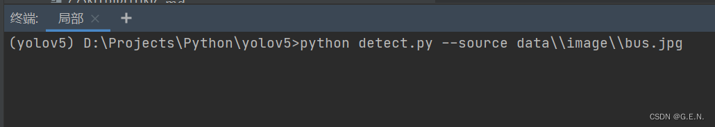
上图的命令中的"--source"参数，对应detect模块中下面的代码

'--source'表示命令后面跟的参数名，type=str表示变量类型为字符串，default表示默认的参数，help参数表示执行help命令时，该参数名显示的帮助信息。

为了更方便理解，我创建了一个test.py 模块

import argparse
# 参数解析器
arg = argparse.ArgumentParser()
# 添加参数
arg.add_argument('--aaa', default='hello world')
arg.add_argument('--bbb', default=123)
# 获取解析的参数
opt = arg.parse_args()
print(opt.aaa, opt.bbb)

命令参数通过arg.pares_args（）函数获取，再通过调用属性的方式获取参数

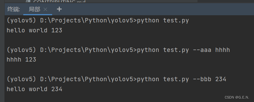
运行结果如上所示。若命令后没有参数名，则参数为默认值；若命令后跟了参数名和参数值，那么这个参数名的值，将会替换为输入的参数值。

yolo v5 的代码正是通过这种方式，将一些重要的参数（如超参数、数据集的路径等）组织起来。在开发阶段，可能不会以这种命令的方式去运行，一般是在部署的时候，才会去用命令去运行。所以开发时若想修改某个参数的值，可以修改这个命令参数名的default关键字参数。

detect模块

接下来就是对 yolo v5 代码的逐句解读

detect模块是对图像、视频、目录、流等进行推断。

导入部分

先看导入部分

"""
Run inference on images, videos, directories, streams, etc.
对图像、视频、目录、流等进行推断。
Usage:
使用
    $ python path/to/detect.py --source path/to/img.jpg --weights yolov5s.pt --img 640
    使用 python 命令运行 detect.py 模块  --source后面跟图片的路径  --weights 后面跟权重文件的路径  --img表示图片的尺寸
"""
import argparse
import os
import sys
from pathlib import Path
import cv2
import numpy as np
import torch
import torch.backends.cudnn as cudnn
"""
确保root目录正确，避免导包时出现错误
因为以下导入的是自定义的包，若根目录错误就会导致导入失败，这里不再过多解释
"""
FILE = Path(__file__).resolve()  # __file__表示当前模块的路径
ROOT = FILE.parents[0]  # YOLOv5 root directory
if str(ROOT) not in sys.path:
    sys.path.append(str(ROOT))  # add ROOT to PATH
ROOT = Path(os.path.relpath(ROOT, Path.cwd()))  # relative
from models.experimental import attempt_load
from utils.datasets import LoadImages, LoadStreams
from utils.general import apply_classifier, check_img_size, check_imshow, check_requirements, check_suffix, colorstr, \
    increment_path, non_max_suppression, print_args, save_one_box, scale_coords, set_logging, \
    strip_optimizer, xyxy2xywh
from utils.plots import Annotator, colors
from utils.torch_utils import load_classifier, select_device, time_sync

中间的代码段是为了确保root目录正确，避免导包时出现错误。若根目录正确，也可省略中间的代码段。导入部分会在使用时再进行讲解。

主函数

接下来暂时跳过函数定义，先看主函数做了哪些操作

if __name__ == "__main__":
    #  接收命令行参数
    opt = parse_opt()
    #  将命令行参数传入main函数
    main(opt)

在主函数中，先调用了parse_opt()函数，用于接收命令行参数

    """
    weight:表示模型的权重参数的路径
    source:表示数据源，可以是图片文件、目录、URL 0为网络摄像头
    imgsz:表示输入图片的大小 默认640*640
    conf-thres:置信度阈值，默认0.25 用于非极大值抑制
    iou-thres:iou阈值，默认0.45 用于非极大值抑制
    max-det:图片最多可以有多少个预测框
    device:程序被装载的位置 CPU或GPU
    view-img:是否展示图片 默认False
    save-text:是否将预测框保存为txt 默认为False
    save-conf: 是否将置信度保存到txt中 默认False
    save-crop: 是否保存裁剪预测框图片, 默认为False
    nosave: 不保存图片、视频 默认False 即保存结果
    classes: 设置只保留某一部分类别, 形如0或者0 2 3
    agnostic-nms: 是否多个类别一起计算nms 默认为False
    augment: 推断时是否进行数据增强 默认为False
    visualize: 是否可视化网络层输出特征 默认为False
    update: 如果为True,则对所有模型进行strip_optimizer操作,去除pt文件中的优化器等信息,默认为False
    project: 保存结果的路径
    name: 保存结果的目录名
    exist_ok: 是否重新结果目录 默认为False
    line-thickness: 画框的线条粗细
    hide-labels: 可视化时隐藏预测类别
    hide-conf: 可视化时隐藏置信度
    half: 是否使用F16精度推理, 半进度提高检测速度
    dnn: 用OpenCV DNN预测
    """

以上为parse_opt()函数中，定义的所有命令行参数及注释。

函数最后返回一个参数对象，所有的命令行参数都在这个对象中，再将这个对象传入mian()函数

main()

def main(opt):
    #  general模块中的函数，用于检查依赖库是否完整
    check_requirements(exclude=('tensorboard', 'thop'))
    #  运行
    run(**vars(opt))

main()函数中只有两行代码，首先调用check_requirements()函数，这是从general模块中导入的函数，用于检查依赖库是否完整。exclude代表排除哪些库，此时函数不会检查这两个库是否存在，因为detect是预测阶段，thsorboard和thop是用于展示训练数据的，预测阶段不需要这两个库。

接下来调用run()函数，vars()函数返回对象的__dict__属性，可以理解为将opt转换为字典，再通过**进行解包，将字典内的键和值作为参数填入run()函数。通过解包的方式，实现了将命令行参数传参至run()函数。

run()

run()函数就是detect模块中进行预测的函数，所有预测工作都在这个函数中完成。

@torch.no_grad()  # 该装饰器表示以下函数内不会进行梯度计算和反向传播
def run(weights=ROOT / 'yolov5s.pt',  # model.pt path(s)

首先注意到run()函数有一个装饰器@torch.no_grad()，装饰器是一种拓展原来函数功能的一种函数。pytorch中的数据格式被称为tensor，用于存储高维数据。tensor中有一个属性为requires_grad，其值为True时，在反向传播的过程中就会计算其梯度，而@torch.no_grad()的作用就是将requires_grad的值置为False，此时便不会计算函数内所有tensor的梯度，有利于节省内存。

run()函数的参数与命令行参数一一对应，这里不再赘述。

接下来对run()函数逐段分析：

资源处理

"""解析资源路径"""
    # 将资源路径路径转换为字符串
    source = str(source)
    # bool类型 是否保存结果  保存（非不保存即为保存） 且 资源路径不以.txt结尾
    save_img = not nosave and not source.endswith('.txt')
    # bool类型 是否为网络摄像头  数据源为数字 或 以.txt结尾 或 小写字母以rtsp://,rtmp://,http://,https://开头
    webcam = source.isnumeric() or source.endswith('.txt') or source.lower().startswith(
        ('rtsp://', 'rtmp://', 'http://', 'https://'))
    # 检查runs/detect目录下的exp目录到exp几了，并增加下一个exp目录，调用general模块中的函数，exist_ok表示只有在路径存在时创建目录
    save_dir = increment_path(Path(project) / name, exist_ok=exist_ok)  # Path类 / 字符串表示在路径后增加一层路径
    # 若保存为txt，返回save/labels  若不保存为txt，则返回save_dir 再创建文件夹  parents：若父目录不存在，创建父目录。exist_ok：只有在目录不存在时创建目录
    (save_dir / 'labels' if save_txt else save_dir).mkdir(parents=True, exist_ok=True)  # make dir

首先是对资源路径进行一些基础判断。判断是否保存结果，以及数据源是否为网络摄像头。接下来就是创建保存的路径。

    # 初始化日志信息
    set_logging()
    # 在控制台上输出YOLO的基本信息 包括当前时间 torch版本 CPU或GPU
    # device表示程序被装载在那块cpu或gpu上
    device = select_device(device)  # select_device()函数是torch_utils中的函数，将程序装载至对应的位置
    # 是否使用半精读计算 需要更少的内存，但需要在支持的GPU上才能运行
    half &= device.type != 'cpu'  # half precision only supported on CUDA

接下来就是初始化日志信息，以及选择将程序装载在哪块cpu或gpu上。

    """加载模型，解析文件后缀"""
    # 若weights参数是一个列表，则返回列表的第一项  否则返回整个weights 这里w为权重文件的路径
    w = str(weights[0] if isinstance(weights, list) else weights)
    # 是否分类，当前后缀名，支持的后缀名
    classify, suffix, suffixes = False, Path(w).suffix.lower(), ['.pt', '.onnx', '.tflite', '.pb', '']
    # 检查后缀名是否支持，否则抛出异常
    check_suffix(w, suffixes)  # check weights have acceptable suffix
    # 将后缀名保存为具体的变量，若这个变量为True,则文件为对应的后缀名
    pt, onnx, tflite, pb, saved_model = (suffix == x for x in suffixes)  # backend booleans
    # 这里的stride和names为临时值  stride为yolo模型中定义的值，为计算的步幅 names为类别标签
    stride, names = 64, [f'class{i}' for i in range(1000)]  # assign defaults

然后就是解析文件的后缀，先判别文件后缀是否合规，再将文件后缀保存为对象，方面后面的判断。

其中stride为特征层级的缩放尺寸，根据YOLO模型的原理，作者将原数据分成了多个大小不同的feature map，每个feature map 感受野不同，可以用于检测不同大小的物体，feature map 越小，模型的感受野越大，可以检测更大的物体，反之同理。stride即为feature map 的缩放尺寸。

    """根据不同的文件后缀，用不同的方式加载模型"""
    # 文件后缀为pt
    if pt:
        # 加载.pt格式的模型 如果文件名中含有torchscript，则通过torch.jit.load(w)加载模型，
        # 否则通过attempt_load(weights, map_location=device)加载模型
        model = torch.jit.load(w) if 'torchscript' in w else attempt_load(weights, map_location=device)
        # 从模型中获取计算的步幅
        stride = int(model.stride.max())  # model stride
        # 从模型中获取分类标签 如果模型中存在module属性，则返回model.module.names 否则返回model.names
        names = model.module.names if hasattr(model, 'module') else model.names  # get class names
        if half:
            # 使用半精读计算
            model.half()  # to FP16
        # 使用两阶段的分类器
        if classify:  # second-stage classifier
            # 加载resnet50作为模型
            modelc = load_classifier(name='resnet50', n=2)  # initialize
            # 将模型装载到对应的位置
            modelc.load_state_dict(torch.load('resnet50.pt', map_location=device)['model']).to(device).eval()
    # 文件后缀为 onnx
    elif onnx:
        # 如果使用opencv加载深度学习模型
        if dnn:
            # check_requirements(('opencv-python>=4.5.4',))
            # 通过opencv加载模型
            net = cv2.dnn.readNetFromONNX(w)
        else:
            # 如果使用opencv加载深度学习模型，则使用onnxruntime库加载
            check_requirements(('onnx', 'onnxruntime'))
            import onnxruntime
            session = onnxruntime.InferenceSession(w, None)
    # 其余的则为tensorflow模型
    else:  # TensorFlow models
        # 检查tensorflow库是否存在
        check_requirements(('tensorflow>=2.4.1',))
        # 导入tensorflow库
        import tensorflow as tf
        # 文件后缀为pb
        if pb:  # https://www.tensorflow.org/guide/migrate#a_graphpb_or_graphpbtxt
            # 以下代码为tensorflow加载pb模型的步骤
            def wrap_frozen_graph(gd, inputs, outputs):
                x = tf.compat.v1.wrap_function(lambda: tf.compat.v1.import_graph_def(gd, name=""), [])  # wrapped import
                return x.prune(tf.nest.map_structure(x.graph.as_graph_element, inputs),
                               tf.nest.map_structure(x.graph.as_graph_element, outputs))
            graph_def = tf.Graph().as_graph_def()
            graph_def.ParseFromString(open(w, 'rb').read())
            frozen_func = wrap_frozen_graph(gd=graph_def, inputs="x:0", outputs="Identity:0")
        # 文件后缀为 saved_model
        elif saved_model:
            # 加载saved_model模型
            model = tf.keras.models.load_model(w)
        # 文件后缀名为 tflite
        elif tflite:
            # 加载tflite模型
            interpreter = tf.lite.Interpreter(model_path=w)  # load TFLite model
            interpreter.allocate_tensors()  # allocate
            input_details = interpreter.get_input_details()  # inputs
            output_details = interpreter.get_output_details()  # outputs
            int8 = input_details[0]['dtype'] == np.uint8  # is TFLite quantized uint8 model
    # 检查图片尺寸 判断图片尺寸是不是模型步长的倍数  若不满足重新计算图片尺寸
    imgsz = check_img_size(imgsz, s=stride)  # check image size

以上的大段代码是根据不同的模型文件，使用不同的方法加载模型。根据代码可以看出，yolo v5 不仅仅支持pytorch的模型，还支持opencv，tensorflow等深度学习库的模型。export模块中也写出了不同模型不同的导出方法。yolo v5 要考虑到系统的兼容性，所以需要兼容这么多格式的模型。但我认为，在实际的使用过程中，这样的代码过于冗杂，只需要兼容一种模型即可。

    # 调用网络摄像头
    if webcam:
        # 检查图片是否可以展示成功
        # 这里通过opencv调用摄像头
        view_img = check_imshow()
        # 优化运行效率
        cudnn.benchmark = True  # set True to speed up constant image size inference
        # 加载流 可以加载网络摄像头甚至Youtube中的视频链接
        dataset = LoadStreams(source, img_size=imgsz, stride=stride, auto=pt)
        bs = len(dataset)  # batch_size
    else:
        # 如果不是网络摄像头，那么加载图片
        dataset = LoadImages(source, img_size=imgsz, stride=stride, auto=pt)
        bs = 1  # batch_size
    # 每个batch_size的vid_path与vide_writer 二维数组 初始化为None
    vid_path, vid_writer = [None] * bs, [None] * bs

上述视频为对数据源的加载，根据webcam判断应该加载视频流或图片。其中LoadStreams与LoadImages均重写了__next__()函数，可以使用for循环进行迭代，将每张照片拿到 。

    # Run inference
    """运行推断过程 将图片带入模型得出结果"""
    if pt and device.type != 'cpu':
        # 带入数据校验模型 使用一张空白的图片进行一次前向推断
        model(torch.zeros(1, 3, *imgsz).to(device).type_as(next(model.parameters())))  # run once
    # 初始化一些中间变量
    dt, seen = [0.0, 0.0, 0.0], 0

接下来执行推断过程，首先要用空白的图片数据带入模型，进行一次前向推断。这个过程可以理解为一个热身的过程，通过热身可以校验模型中数据的维度等是否正确。这是一种训练技巧。

for循环

    # 从图片或视频加载每一张图片
    # 每张图片的推断过程均在for循环内完成
    # path为图片的路径 img为resize处理后的图片 im0s表示未处理的原图 vid_cap为视频流实例
    for path, img, im0s, vid_cap in dataset:
        """处理图片"""
        # 获取cpu上执行的时间
        t1 = time_sync()
        # 如果模型为onnx格式
        if onnx:
            # 将图片数组中的元素改为float32
            img = img.astype('float32')
        # 若模型不为onnx
        else:
            # 把图片数组装载在对应的cpu或gpu上
            img = torch.from_numpy(img).to(device)
            # 如果使用半精读计算 就将数据转为半精读 否则还是float
            img = img.half() if half else img.float()  # uint8 to fp16/32
        # /255.0将数据映射至0-1之间 归一化处理
        img = img / 255.0  # 0 - 255 to 0.0 - 1.0
        # 若图片为三维
        if len(img.shape) == 3:
            # 为图片扩展一个维度 batch_size的维度
            img = img[None]  # expand for batch dim
        # 获取结束时间
        t2 = time_sync()
        # 将时间累积
        dt[0] += t2 - t1

接下来就是通过for循环，将每张照片从流或文件夹中获取出来，每执行一次for循环就是完成一次对图片的推断，对于这张图片的推断均体现在for循环内。这里先截取了for循环的一部分，首先是对图片的处理，将图片数组进行归一化，并修改维度。

# Inference
        """推断过程 不同模型通过不同方式得出预测结果"""
        # 若模型为pt格式
        if pt:
            # visualize为可视化，默认为False,若进行可视化就新建目录，并保存结果，否则返回false
            visualize = increment_path(save_dir / Path(path).stem, mkdir=True) if visualize else False
            # 获取预测结果，并保存第一维度为pred
            # pred为预测的结果 shape为(1,18900,85)
            pred = model(img, augment=augment, visualize=visualize)[0]
        # 若模型为onnx格式
        elif onnx:
            # 若使用opencv的深度学习
            if dnn:
                # 输入模型
                net.setInput(img)
                # 获取结果
                pred = torch.tensor(net.forward())
            else:
                # 获取预测结果
                pred = torch.tensor(session.run([session.get_outputs()[0].name], {session.get_inputs()[0].name: img}))
        # 使用tensorflow模型
        else:  # tensorflow model (tflite, pb, saved_model)
            imn = img.permute(0, 2, 3, 1).cpu().numpy()  # image in numpy
            if pb:
                # 获取pb模型的预测结果
                pred = frozen_func(x=tf.constant(imn)).numpy()
            elif saved_model:
                # 获取save_model模型的预测结果
                pred = model(imn, training=False).numpy()
            elif tflite:
                # 获取tflite模型的预测结果
                if int8:
                    scale, zero_point = input_details[0]['quantization']
                    imn = (imn / scale + zero_point).astype(np.uint8)  # de-scale
                interpreter.set_tensor(input_details[0]['index'], imn)
                interpreter.invoke()
                pred = interpreter.get_tensor(output_details[0]['index'])
                if int8:
                    scale, zero_point = output_details[0]['quantization']
                    pred = (pred.astype(np.float32) - zero_point) * scale  # re-scale
            # pred[..., 0]这样的语法表示抽取数组的第几列，作为一个tensor    
            pred[..., 0] *= imgsz[1]  # x
            pred[..., 1] *= imgsz[0]  # y
            pred[..., 2] *= imgsz[1]  # w
            pred[..., 3] *= imgsz[0]  # h
            pred = torch.tensor(pred)

上述代码将图片输入不同的模型，并得到预测结果。将data/images/bus.jpg图片输入模型，得到的是一个shape为（1，18900，85）的tensor；将data/images/zidane.jpg输入模型，齐达内的图片得到的是一个shape为（1，15120，85）的tensor。

1表示batch_size，表示这个batch_size中只有一张图片的预测结果，因为输入模型的batch_size就是1，所以输出的结果也为1。

18900或15120表示模型预测出了1890或15120个预测框。

85表示每个预测框中含有4个位置信息（包括预测框的x，y，w，h）、一个置信度信息和coco数据集80个类别的条件概率信息。

        # NMS 非极大值抑制 pred为预测结果, conf_thres为置信度阈值 默认为0.25  iou_thres为iou阈值 默认为0.45
        # classes为是否只保留特定的类别 默认为None  agnostic_nms True表示多个类一起计算nms，False表示按照不同的类分别进行计算nms
        # max_det为保留的最大检测框数 默认为1000 也就是一张图片最多检测1000个物体
        # 经过极大值抑制后 shape变为(1,5,6) 1表示batch_size 5表示共有5个预测框 6表示x,y,x,y两个坐标，1个类别概率，1个类别索引
        pred = non_max_suppression(pred, conf_thres, iou_thres, classes, agnostic_nms, max_det=max_det)
        dt[2] += time_sync() - t3

有了预测结果，接下来要从预测出的18900个预测框中筛选出最合适的框，这个过程被称为非极大值抑制。

def non_max_suppression(prediction, conf_thres=0.25, iou_thres=0.45, classes=None, agnostic=False, multi_label=False,
                        labels=(), max_det=300):
    """Runs Non-Maximum Suppression (NMS) on inference results
    Returns:
         list of detections, on (n,6) tensor per image [xyxy, conf, cls]
    """
    # 获取类别数
    nc = prediction.shape[2] - 5  # number of classes
    # prediction[..., 4] 表示数据的第四列，这里指置信度
    # 判断每一位的置信度是否大于置信度阈值 返回一个shape为(1，18900)的bool类型的tensor，代表这一位是否大于置信度阈值
    xc = prediction[..., 4] > conf_thres  # candidates
    # Checks 检测阈值是否合法
    assert 0 <= conf_thres <= 1, f'Invalid Confidence threshold {conf_thres}, valid values are between 0.0 and 1.0'
    assert 0 <= iou_thres <= 1, f'Invalid IoU {iou_thres}, valid values are between 0.0 and 1.0'
    # Settings
    min_wh, max_wh = 2, 4096  # (pixels) minimum and maximum box width and height
    max_nms = 30000  # maximum number of boxes into torchvision.ops.nms()
    time_limit = 10.0  # seconds to quit after
    redundant = True  # require redundant detections
    multi_label &= nc > 1  # multiple labels per box (adds 0.5ms/img)
    merge = False  # use merge-NMS
    t = time.time()
    # 定义输出数据
    output = [torch.zeros((0, 6), device=prediction.device)] * prediction.shape[0]
    # xi表示第几个batch x表示这个batch内所有预测框
    for xi, x in enumerate(prediction):  # image index, image inference
        # Apply constraints
        # x[((x[..., 2:4] < min_wh) | (x[..., 2:4] > max_wh)).any(1), 4] = 0  # width-height
        # xi为0 表示第0个batch
        # xc[xi] 表示获取这个batch内所有的置信度是否大于置信度阈值
        # 这种表示方式为x[xc[xi]] 将x中为True的值取出，并赋值给x
        # x现在表示，18900个预测框置信度中大于置信度阈值的预测框 shape为(52, 85)
        # 此时根据置信度阈值的过滤，预测框只剩下18900个
        x = x[xc[xi]]  # confidence
        # Cat apriori labels if autolabelling
        # 暂时不理解
        if labels and len(labels[xi]):
            l = labels[xi]
            v = torch.zeros((len(l), nc + 5), device=x.device)
            v[:, :4] = l[:, 1:5]  # box
            v[:, 4] = 1.0  # conf
            v[range(len(l)), l[:, 0].long() + 5] = 1.0  # cls
            x = torch.cat((x, v), 0)
        # If none remain process next image
        # 若预测框数为0，则处理下一个batch
        if not x.shape[0]:
            continue
        # Compute conf
        # x[:, 5:] = x[:, 5:] * x[:, 4:5]
        # 80个类别的概率为条件类别概率，是假设这个框内有物体的情况下，该物体是某一类的概率
        # 置信度可以理解为预测框内存在物体的概率
        # 将所有类别的条件类别概率与置信度相乘才是某个类别的真正概率
        # 经过计算，物体的条件类别概率被计算为了真正的概率
        x[:, 5:] *= x[:, 4:5]  # conf = obj_conf * cls_conf
        # Box (center x, center y, width, height) to (x1, y1, x2, y2)
        # 将x,y,w,h （一个坐标和一个宽一个高） 的表示方法改为 x,y,x,y（两个坐标，矩形的左上角和右下角）表示
        box = xywh2xyxy(x[:, :4])
        # Detections matrix nx6 (xyxy, conf, cls)
        if multi_label:
            i, j = (x[:, 5:] > conf_thres).nonzero(as_tuple=False).T
            x = torch.cat((box[i], x[i, j + 5, None], j[:, None].float()), 1)
        # 每个类只标一个标签
        else:  # best class only
            # conf为最大的类别概率，j为最大类别概率的索引值
            conf, j = x[:, 5:].max(1, keepdim=True)
            # 将结果拼到一起
            # box shape为(52, 4) 表示52个预测框的xyxy坐标表示
            # conf shape为(52, 1) 表示52个预测框的最大类别概率
            # j shape为(52,1) 表示最大类别概率的索引值，用于表示哪个类别
            # 此时x的shape为(52, 6)
            x = torch.cat((box, conf, j.float()), 1)[conf.view(-1) > conf_thres]
        # Filter by class
        if classes is not None:
            x = x[(x[:, 5:6] == torch.tensor(classes, device=x.device)).any(1)]
        # Apply finite constraint
        # if not torch.isfinite(x).all():
        #     x = x[torch.isfinite(x).all(1)]
        # Check shape
        n = x.shape[0]  # number of boxes
        # 如果没有box 执行下一张图片的推断
        if not n:  # no boxes
            continue
        # 如果预测框的个数大于了最大值
        # 这里的预测框个数指的不是最终预测的个数
        elif n > max_nms:  # excess boxes
            # 根据概率值排序
            x = x[x[:, 4].argsort(descending=True)[:max_nms]]  # sort by confidence
        # Batched NMS
        # agnostic参数 True表示多个类一起计算nms，False表示按照不同的类分别进行计算nms
        # 这里的c为偏移量 若不同的类分别进行计算nms，就把类别的索引乘一个很大的值
        c = x[:, 5:6] * (0 if agnostic else max_wh)  # classes
        # boxes为原来的box加上c偏置量 这样做是为了确保不同类别的预测框不会重叠
        # scores为类别的概率值
        boxes, scores = x[:, :4] + c, x[:, 4]  # boxes (offset by class), scores
        # 执行非极大值抑制
        # 这里的非极大值抑制是torchvision中实现的非极大值抑制
        # nms的原理为计算不同预测框的iou（交并比），若大于阈值，则判定两个预测框预测了同一物体
        # 通过这种方式筛出预测框 返回最后确定的预测框索引
        i = torchvision.ops.nms(boxes, scores, iou_thres)  # NMS
        # 如果最后的预测框数量大于最大预测数
        if i.shape[0] > max_det:  # limit detections
            # 只取到最大预测数
            i = i[:max_det]
        if merge and (1 < n < 3E3):  # Merge NMS (boxes merged using weighted mean)
            # update boxes as boxes(i,4) = weights(i,n) * boxes(n,4)
            iou = box_iou(boxes[i], boxes) > iou_thres  # iou matrix
            weights = iou * scores[None]  # box weights
            x[i, :4] = torch.mm(weights, x[:, :4]).float() / weights.sum(1, keepdim=True)  # merged boxes
            if redundant:
                i = i[iou.sum(1) > 1]  # require redundancy
        # output为先前定义的空白结果
        # 让output[xi]目的是使输出结果的batch与输入相对应
        # x[i]表述从x中取出i中的索引
        output[xi] = x[i]
        # 非极大值抑制过程时间超时
        if (time.time() - t) > time_limit:
            print(f'WARNING: NMS time limit {time_limit}s exceeded')
            break  # time limit exceeded
    # 返回结果 output的shape为(1,5,6)
    return output

非极大值抑制是yolo在处理预测结果时的重要环节，所以这里把非极大值抑制的代码解读也写出来，非极大值抑制主要分为两个步骤。

第一步为过滤低置信度预测框。置信度反应了该预测框中存在对象的概率。经过模型的推断，产生了18900个预测框，过滤掉低置信度的预测框后，仅剩52个预测框，而剩下的52个预测框，大多数都是多个预测框预测了同一个物体，这时便要进行第二步。

第二步为通过IOU阈值过滤。首先把不同类别的预测框加上不同的偏置量，保证不同类别的预测框不会有重叠。然后计算每个类别预测框的IOU，若两个预测框的IOU大于给定阈值，那么就判定这两个预测框预测了同一个的对象，并只保留一个类别概率大的框。

        # Second-stage classifier (optional)
        if classify:
            pred = apply_classifier(pred, modelc, img, im0s)
        # Process predictions
        # i表示 batch det表示五个预测框
        for i, det in enumerate(pred):  # per image
            # seen 为计数
            seen += 1
            # 如果数据源是网络摄像头
            if webcam:  # batch_size >= 1
                p, s, im0, frame = path[i], f'{i}: ', im0s[i].copy(), dataset.count
            # 数据源不是网络摄像头
            else:
                p, s, im0, frame = path, '', im0s.copy(), getattr(dataset, 'frame', 0)
            # 设置保存路径
            p = Path(p)  # to Path
            save_path = str(save_dir / p.name)  # img.jpg
            txt_path = str(save_dir / 'labels' / p.stem) + ('' if dataset.mode == 'image' else f'_{frame}')  # img.txt
            # 设置打印图片的信息
            s += '%gx%g ' % img.shape[2:]  # print string
            gn = torch.tensor(im0.shape)[[1, 0, 1, 0]]  # normalization gain whwh
            # 保存图片
            imc = im0.copy() if save_crop else im0  # for save_crop
            # 绘图类实例
            annotator = Annotator(im0, line_width=line_thickness, example=str(names))
            # 如果有预测框
            if len(det):
                # Rescale boxes from img_size to im0 size
                # 映射图片的尺寸
                det[:, :4] = scale_coords(img.shape[2:], det[:, :4], im0.shape).round()
                # Print results
                # 输出结果
                for c in det[:, -1].unique():
                    n = (det[:, -1] == c).sum()  # detections per class
                    s += f"{n} {names[int(c)]}{'s' * (n > 1)}, "  # add to string
                # Write results
                # 保存结果
                for *xyxy, conf, cls in reversed(det):
                    # 保存txt文件
                    if save_txt:  # Write to file
                        # 将坐标转换为旧的格式
                        xywh = (xyxy2xywh(torch.tensor(xyxy).view(1, 4)) / gn).view(-1).tolist()  # normalized xywh
                        line = (cls, *xywh, conf) if save_conf else (cls, *xywh)  # label format
                        # 将预测结果写入文件 路径默认为“runs\detect\exp*\labels”
                        with open(txt_path + '.txt', 'a') as f:
                            f.write(('%g ' * len(line)).rstrip() % line + '\n')
                    if save_img or save_crop or view_img:  # Add bbox to image
                        c = int(cls)  # integer class
                        # 获取类别标签
                        label = None if hide_labels else (names[c] if hide_conf else f'{names[c]} {conf:.2f}')
                        # 绘制含有标签的边框
                        annotator.box_label(xyxy, label, color=colors(c, True))
                        # 将预测框内的图片单独保存
                        if save_crop:
                            save_one_box(xyxy, imc, file=save_dir / 'crops' / names[c] / f'{p.stem}.jpg', BGR=True)
            # Print time (inference-only)
            print(f'{s}Done. ({t3 - t2:.3f}s)')
            # Stream results
            # im0为绘制好的图片
            im0 = annotator.result()
            # 如果显示该图片
            if view_img:
                cv2.imshow(str(p), im0)
                cv2.waitKey(1)  # 1 millisecond
            # Save results (image with detections)
            # 保存绘制完的图片
            if save_img:
                # 若为图片
                if dataset.mode == 'image':
                    # 向路径中保存图片
                    cv2.imwrite(save_path, im0)
                # 是视频或者流
                else:  # 'video' or 'stream'
                    if vid_path[i] != save_path:  # new video
                        vid_path[i] = save_path
                        if isinstance(vid_writer[i], cv2.VideoWriter):
                            vid_writer[i].release()  # release previous video writer
                        if vid_cap:  # video
                            fps = vid_cap.get(cv2.CAP_PROP_FPS)
                            w = int(vid_cap.get(cv2.CAP_PROP_FRAME_WIDTH))
                            h = int(vid_cap.get(cv2.CAP_PROP_FRAME_HEIGHT))
                        else:  # stream
                            fps, w, h = 30, im0.shape[1], im0.shape[0]
                            save_path += '.mp4'
                        # 最后保存为视频
                        vid_writer[i] = cv2.VideoWriter(save_path, cv2.VideoWriter_fourcc(*'mp4v'), fps, (w, h))
                    vid_writer[i].write(im0)

接下来的内容就比较简单了，首先将预测款绘制在图片上，然后将图片保存。此时for循环结束

输出结果

    # Print results
    t = tuple(x / seen * 1E3 for x in dt)  # speeds per image
    print(f'Speed: %.1fms pre-process, %.1fms inference, %.1fms NMS per image at shape {(1, 3, *imgsz)}' % t)
    if save_txt or save_img:
        s = f"\n{len(list(save_dir.glob('labels/*.txt')))} labels saved to {save_dir / 'labels'}" if save_txt else ''
        print(f"Results saved to {colorstr('bold', save_dir)}{s}")
    if update:
        strip_optimizer(weights)  # update model (to fix SourceChangeWarning)

最后将结果输出在控制台，detect模块到此结束。

其他的几个模块后续更新。