
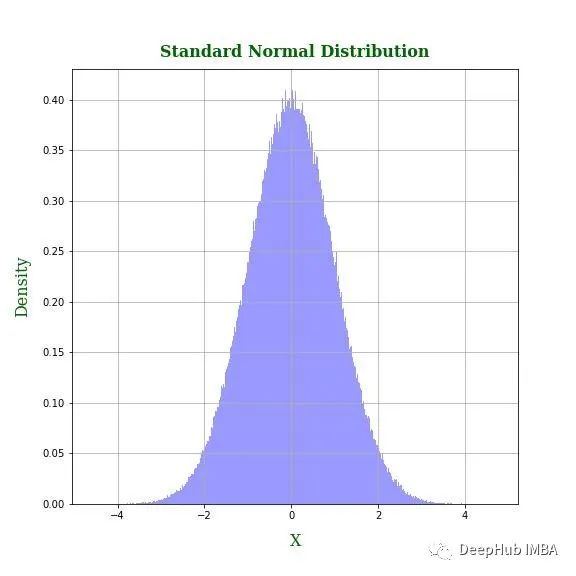
正态(高斯)分布在机器学习中起着核心作用,线性回归模型中要假设随机误差等方差并且服从正态分布,如果变量服从正态分布,那么更容易建立理论结果。
统计学领域的很大一部分研究都是假设数据是正态分布的,所以如果我们的数据具有是正态分布,那么么则可以获得更好的结果。但是一般情况下我们的数据都并不是正态分布,所以 如果我们能将这些数据转换成正态分布那么对我们建立模型来说是一件非常有帮助的事情。
 standard_normal = np.random.normal(0, 1, size=1_000_000)
 fontdict = {'family':'serif', 'color':'darkgreen', 'size':16}
 fig, axs = plt.subplots(1, 1, figsize=(8, 8))
 axs.hist(standard_normal, bins=1000, density=True, fc=(0,0,1,0.4))

 axs.set_title('Standard Normal Distribution', fontdict=fontdict, fontweight='bold', pad=12)
 axs.set_xlabel('X', fontdict=fontdict, fontweight='normal', labelpad=12)
 axs.set_ylabel('Density', fontdict=fontdict, fontweight='normal', labelpad=12)
 axs.grid()
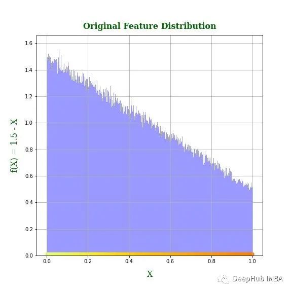
如果你正在处理一个密度(大约)呈线性下降的特性(见下图)。
 x = np.linspace(0, 1, 1001)
 sample = (3 - np.sqrt(9 - 8 * np.random.uniform(0, 1, 1_000_000))) / 2fontdict = {'family':'serif', 'color':'darkgreen', 'size':16}
 fig, axs = plt.subplots(1, 1, figsize=(8, 8))
 axs.hist(sample, bins=1000, density=True, fc=(0,0,1,0.4))
 axs.scatter(x, np.full_like(x, 0.01), c=x, cmap=cmap)
 axs.set_title('Original Feature Distribution', fontdict=fontdict, fontweight='bold', pad=12)
 axs.set_xlabel('X', fontdict=fontdict, fontweight='normal', labelpad=12)
 axs.set_ylabel('Density', fontdict=fontdict, fontweight='normal', labelpad=12)
 axs.grid()
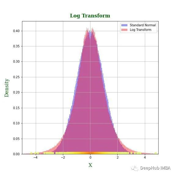
要将这个特征转换为具有钟形分布的变量,可能没有那么简单,我如果我使用某种变换将密度最高的左端放到中心,那么中心两侧的其余点怎么办?
如果变换是将点从中间和右边的[0,1]移到均值的任意一边(N(0,1) =0)那么本质上是一个非单调的变换,这不是很好因为那样的话,变换后的特征值就没有什么意义了。虽然我们能够得到一个钟形分布,但是对转换后的值没有意义,排序也不再被保留(见下图3中转换后的特征值的散点图)。
 log_transform = lambda ar: np.multiply(1.6 * np.log10(ar+1e-8), np.random.choice((-1, 1), size=ar.size)
 fontdict = {'family':'serif', 'color':'darkgreen', 'size':16}
 fig, axs = plt.subplots(1, 1, figsize=(8, 8))
 axs.hist(standard_normal, bins=1_000, density=True, fc=(0,0,1,0.4), label='Standard Normal')
 axs.hist(log_transform(sample), bins=1_000, density=True, fc=(1,0,0,0.4), label='Log Transform')

 axs.scatter(log_transform(x), np.full_like(x, 3e-3), c=x, cmap=cmap)
 axs.set_xlim(-5, 5)
 axs.set_title('Log Transform', fontdict=fontdict, fontweight='bold', pad=12)
 axs.set_xlabel('$\pm$1.6log(X)', fontdict=fontdict, fontweight='normal', labelpad=12)*
 axs.set_ylabel('Density', fontdict=fontdict, fontweight='normal', labelpad=12)

 axs.legend()
 axs.grid()
特征的密度是单调递减的。目标是使用范围(-∞,∞)的变换来拉伸和压缩不同点周围的[0,1]范围,并且变换空间中每个点的密度应该是N(0,1)所给出的。所以是不是可以尝试使用其他的方法呢?
先看看原始特征的CDF函数
如果确保变换函数将原始分布的 (i-1)ᵗʰ 和 iᵗʰ 百分位数之间的点映射到 N( 0,1)那会怎么样呢?

g 是我们正在寻找的变换,Φ 是 N(0,1) 的 CDF
但是这可能只是最终目标只是这种方法的延伸。因为我们的方法不应限制在由百分位数定义的区间,而是想要一个函数,它可以满足上面原始CDF公式中的每个区间的要求。于是就得到了下面的公式

如果你对概率论比较熟悉,那么回想一下概率的特征在于它的分布函数(Jean Jacod 和 Philip Protter 的 Probability Essentials 中的定理 7.1)。我将把自己限制在了单调递增函数的空间中。

单调递增函数的约束假设集,如果我能找到一个函数使变换后的特征的CDF等于N(0,1)的CDF,那不就可以了吗。这与上面公式中的单调递增约束一起,得到了下面的公式。
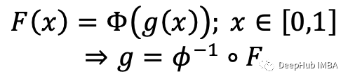
将函数g变换为Φ的逆函数和F的复合函数
下面看看结果,我们使用上面总结的结果来转的特征,使其具有标准正态分布。
 fontdict = {'family':'serif', 'color':'darkgreen', 'size':16}
 fig, axs = plt.subplots(1, 1, figsize=(8, 8))
 axs.hist(standard_normal, bins=1_000, density=True, fc=(0,0,1,0.4), label='Standard Normal')
 axs.hist(scipy.stats.norm.ppf(1.5*sample - 0.5*(sample**2)), bins=1000, density=True, fc=(1,0,0,0.4), label='Equation 4 Transform')
 axs.scatter(norm.ppf(1.5*x - 0.5*(x**2)), np.full_like(x, 3e-3), c=x, cmap=cmap)

 axs.set_xlim(-5, 5)
 axs.set_title("Transformed Feature's Density", fontdict=fontdict, fontweight='bold', pad=12)
 axs.set_xlabel('$\Phi^{-1}(F$(X))', fontdict=fontdict, fontweight='normal', labelpad=12)
 axs.set_ylabel('Density', fontdict=fontdict, fontweight='normal', labelpad=12)

 axs.legend()
 axs.grid()
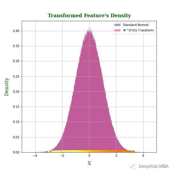
任何分布(只要它是一个连续分布函数)都可以使用这个方法。但是在使用它之前,还是需要看看用例中使用它是否有意义。
 fontdict = {'family':'serif', 'color':'darkgreen', 'size':16}
 fig, axs = plt.subplots(1, 1, figsize=(8, 8))
 axs.scatter(x, norm.ppf(1.5*x - 0.5*(x**2)), c=x, cmap=cmap)

 axs.set_xlim(0, 1)
 axs.set_title('Transform', fontdict=fontdict, fontweight='bold', pad=12)
 axs.set_xlabel('X', fontdict=fontdict, fontweight='normal', labelpad=12)
 axs.set_ylabel('$\Phi^{-1}(F$(X))', fontdict=fontdict, fontweight='normal', labelpad=12)
 axs.grid()
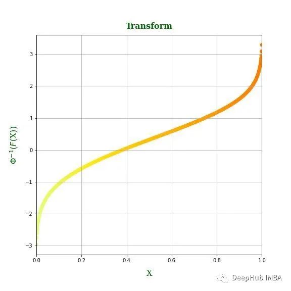
我们的转函数看起来是这样的,这个过程给出了如图5所示的转换。需要注意的是:这个特征取值接近 0 或接近 1 时输出波动大,但当值接近 0.5 时输出波动小。如果不是这种情况会给模型提供对特征的错误解释,可能会损害其性能。
作者:Jasraj Singh