
Astar和IDAstar搜索算法解决十五数码(15-puzzle)问题
(文末附实现代码,此前为理论与具体问题分析)
文章目录
一、实验题目:
利用A搜索算法和IDA搜索算法解决15-puzzle问题
实验测例包括(以列表表示):
Example1:[[1, 15, 7, 10],[9, 14, 4, 11], [8, 5,0 , 6],[13, 3, 2, 12]]
Example2: [[1, 7, 8, 10],[6, 9, 15, 14], [13, 3, 0, 4], [11, 5, 12, 2]]
Example3: [[5, 6, 4, 12], [11, 14, 9, 1], [0, 3, 8, 15], [10, 7, 2, 13]]
Example4: [[14, 2, 8, 1], [7, 10, 4, 0], [6, 15, 11, 5], [9, 3, 13, 12]]
额外50步以上测例:
测例1: [[11, 3, 1, 7], [4, 6 ,8 ,2], [15 ,9 ,10, 13], [14, 12, 5 ,0]]
测例2: [[14, 10, 6, 0], [4, 9 ,1 ,8], [2, 3, 5 ,11], [12, 13, 7 ,15]]
测例3: [[14, 10, 6, 0],[4, 9 ,1 ,8],[2, 3, 5 ,11],[12, 13, 7 ,15]]
测例4: [[6 ,10, 3, 15],[14, 8, 7, 11],[5, 1, 0, 2],[13, 12, 9 ,4]]
二、实验内容
本次实验主要针对两种启发式搜索进行实现 A搜索算法和IDA搜索算法。
启发式搜索与盲目搜索或者无信息搜索最大的区别就在于启发式搜索采用了启发信息来引导整个搜索的过程,能够减少搜索的范围,降低求解问题的复杂度。这里的启发信息主要由估价函数组成,估价函数f(x)由两部分组成,从初始结点到当前结点n所付出的实际代价g(n)和从当前结点n到目标结点的最优路径的代价估计值h(n),即
     f


     (


     n


     )


     =


     g


     (


     n


     )


     +


     h


     (


     n


     )


    f(n) = g(n) + h(n)


 f(n)=g(n)+h(n)
启发式函数设计:
启发式函数需要满足以下两种性质:
1.可采纳的(admissible)
     定


     义


     h


     (


     n


     )


     为


     到


     终


     点


     代


     价


     的


     预


     估


     值


     ,


      h


      ∗


     (


     n


     )


     为


     真


     实


     的


     代


     价


     定义h(n)为到终点代价的预估值,h^{*}(n)为真实的代价


 定义h(n)为到终点代价的预估值,h∗(n)为真实的代价


     若


     h


     (


     n


     )


     <


     =


      h


      ∗


     (


     n


     )


     成


     立


     ,


     即


     预


     估


     值


     小


     于


     真


     实


     值


     的


     时


     候


     ,


     算


     法


     必


     然


     可


     以


     找


     到


     一


     条


     最


     短


     路


     径


     若h(n)<=h^{*}(n)成立,即预估值小于真实值的时候,算法必然可以找到一条最短路径


 若h(n)<=h∗(n)成立,即预估值小于真实值的时候,算法必然可以找到一条最短路径
2.单调的(consistent)
     h


     (


     n


     )


     <


     =


     h


     (


      n


       ′


     )


     +


     c


     o


     s


     t


     (


     n


     ,


      n


       ′


     )


     h(n)<=h(n^{'})+cost(n,n^{'})


 h(n)<=h(n′)+cost(n,n′)
算法原理:
I. A*算法
A*搜索算法与BFS类似,但它需要加入估价函数作为启发信息。
算法步骤
- 开始
1.从起点A开始,将其当作待处理的结点加入open表中
2.将其子结点也加入open表中,计算f(x), g(x),h(x),其中f(x)=g(x)+h(x),g(x)表示当前结点的代价,h(x)为当前结点到达目标的代价的估计
3.从open表中取出结点A,并将其加入close表中,表示已经扩展过
- 循环
4.从open表中弹出f(x)最小的结点C,并加入close表中
5.将C的子结点加入到open表中
6.如果待加入open表中的结点已经在open表中,则更新它们的g(x),保持open表中该结点的g(x)最小
II. IDA*算法
算法步骤:
算法基于深度优先搜索的思想,加入启发信息,对于给定的阈值bound,定义递归过程
- 从开始结点C,计算所有子结点的f(x),选取最小的结点作为下一个访问结点
- 对于某个节点,如果其f(x)大于bound,则返回当前结点的f(x),取当中最小的f(x)对bound进行更新
- 进行目标检测
三、实验结果及分析
【注:实验结果文件均保存于result文件夹中,其中包含搜索的路径,探索的结点个数,运行时间以及IDAstar的搜索限制值】
1.启发式函数
选取不同的启发式函数会对算法的效率造成一定程度的影响,现针对两种启发式函数进行分析。
启发式函数1: 错置的数码块个数之和
在这个启发式函数中,需要统计当前状态下被错置的数码块之和,其值作为当前状态的H(x)。
启发式函数2: 曼哈顿距离
在这个启发式函数中,利用曼哈顿距离公式
     M


     =


     a


     b


     s


     (


     n


     o


     d


     e


     .


     x


     −


     g


     o


     a


     l


     .


     x


     )


     +


     a


     b


     s


     (


     n


     o


     d


     e


     .


     y


     −


     g


     o


     a


     l


     .


     y


     )


    M = abs(node.x - goal.x) + abs(node.y - goal.y)


 M=abs(node.x−goal.x)+abs(node.y−goal.y)
对除了数码块0以外的所有数码块计算其曼哈顿距离,并将其累加作为当前状态的总曼哈顿距离,
注:计算曼哈顿距离时之所以排除数码块0,是因为若考虑数码块0,则不满足可采纳性(Admittable)
     h


     (


     n


     )


     <


     =


      h


      ∗


     (


     n


     )


    h(n)<=h^{*}(n)


 h(n)<=h∗(n),这个启发式函数就不满足算法的最优性。
举个简单的例子来证明这个结论,若现在的状态为如下: 那么下一步肯定是将数码块0向右移动一格,也就是代价为1, 而当前状态的
     h


     (


     n


     )


     =


     2


    h(n) = 2


 h(n)=2,也就是说


     h


     (


     n


     )


     >


      h


      ∗


     (


     n


     )


    h(n)>h^{*}(n)


 h(n)>h∗(n), 这就与可采纳性矛盾。
1 2 3 4
5 6 7 8
9 10 11 12
13 14 0 15
启发式函数1和启发式函数2的效率比较:
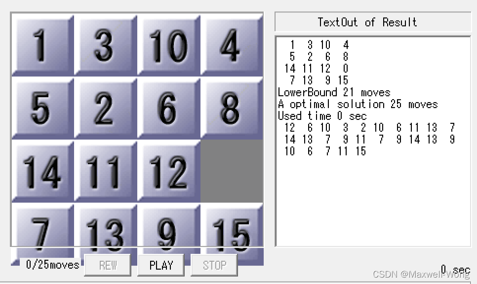
为了比较这两种启发式函数的效率,并且获得具体的数值,现采用25步的测例进行实验。
关键代码:
(1)启发式函数1:

(2)启发式函数2:

运行结果:
在A*搜索算法上:
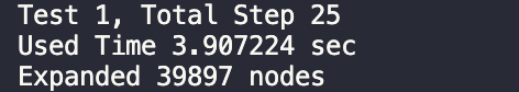
启发式函数1:
启发式函数2:
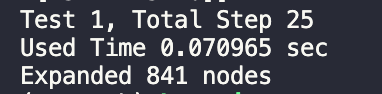
从结果可以看出,采用启发式函数1需要扩展更多的结点,且运行时间更慢。
因此,在之后的实验中,均采用曼哈顿距离作为启发式函数。
2.环检测优化
- A搜索算法***优化说明:在A搜索算法中维护的close表起到了环检测的作用,将扩展过的结点加入到close表中,在每次需要扩展新的结点的时候查找在close表中有没有出现,若没有出现,则将其加入到open表中,作为待扩展结点。因此,我们要针对close表进行优化,达到以更优的效率进行查表。实现方法:以set容器作为close表的数据结构,将数码矩阵状态转换成字符串,再通过python内置的hash函数转换成唯一的哈希值。*优化原理: 对比list,以set容器作为close表存储状态的数据结构性能更优,基于针对close表的操作只有插入和查表两种操作,在查找的性能方面set肯定是优于list;实践是检验真理的唯一标准,我们针对list和set对于查找的性能做一个简单的实验以下是在list和set中找出随机数是否存在其相反数。

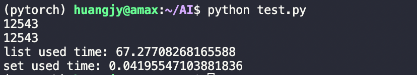 从结果可以看出,set在50000个数据中查找的速度是list的1640倍。在这种情况下,如果选择使用list作为close表,效率可想而知是不如set的。关键代码:此处
 CLOSE = set()close表定义为set容器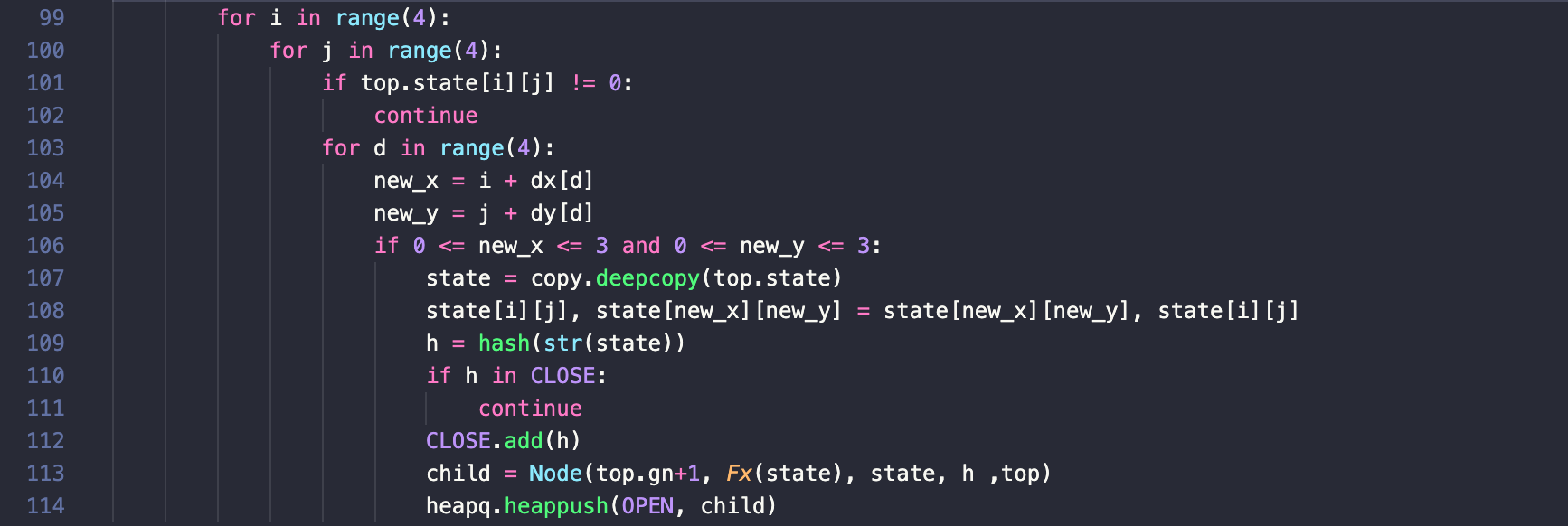 在代码中,将生成的子结点的状态转换成字符串,再通过hash函数(hash函数只能以字符串、数字、字典、集合作为参数)获取其哈希值存到close表中, 在第110行中就用到了查表,如果close表中不存在该结点,则将其加入到close表中。
 - IDA*搜索算法IDA搜索算法本质上为深度优先搜索算法,它在空间上有比广度优先算法更优的性能,即 O ( b m ) O(bm) O(bm) (其中b是后继结点的个数,m是搜索树的深度),因为它不需要使用队列来保存已经拓展过的结点,如果IDA 采用了环检测则会破坏它在空间上的最优性。因此,对于IDA*的优化并没有采用环检测,而是采用路径检测(这将会在之后讨论到)
3.A与IDA算法性能的比较
启发式函数:曼哈顿距离
数码状态存储数据结构:List
环检测数据结构:Set
4.实验结果
(运行结果路径可在Github仓库中的Results文件下载)
测例1 [[1, 15, 7, 10],[9, 14, 4, 11], [8, 5,0 , 6],[13, 3, 2, 12]]

A* 搜索算法运行结果:
Test 1, Total Step 40
Used Time 0.303069 sec
Expanded 2765 nodes
IDA* 搜索算法运行结果:
Test 1, Total Step 40
Used Time 1.194115 sec
Expanded 25590 nodes
Bound: 40
测例2 [[1, 7, 8, 10],[6, 9, 15, 14], [13, 3, 0, 4], [11, 5, 12, 2]]

A* 搜索算法运行结果:
Test 2, Total Step 40
Used Time 0.130206 sec
Expanded 4009 nodes
IDA* 搜索算法运行结果:
Test 2, Total Step 40
Used Time 0.526660 sec
Expanded 6348 nodes
Bound: 40
测例3 [[5, 6, 4, 12], [11, 14, 9, 1], [0, 3, 8, 15], [10, 7, 2, 13]]

A* 搜索算法运行结果:
Test 3, Total Step 40
Used Time 0.089238 sec
Expanded 575 nodes
IDA* 搜索算法运行结果:
Test 3, Total Step 40
Used Time 0.241839 sec
Expanded 2602 nodes
Bound: 40
测例4 [[14, 2, 8, 1], [7, 10, 4, 0], [6, 15, 11, 5], [9, 3, 13, 12]]

A* 搜索算法运行结果:
Test 4, Total Step 40
Used Time 0.985068 sec
Expanded 15017 nodes
IDA* 搜索算法运行结果:
Test 4, Total Step 40
Used Time 18.741641 sec
Expanded 252281 nodes
Bound: 40
总结:
测例Example1Example2Example3Example4Used Time [A*| IDA*]0.30|1.190.13|0.520.06|0.240.98|18.74Expanded Nodes [A* | IDA*] (nodes)2765 | 255904009 |6348575|260215017|252281Better [A* | IDA*]AAAA
从以上A* 与IDA在深度为40的搜索树的表现情况来看,A的搜索效率大于IDA,此外,从扩展的结点个数来看,IDA 扩展的结点数更多,这跟IDA本身搜索的方式有关。 由于A 需要保存扩展过的结点,因此内存消耗远大于IDA* ,至此,可以猜测IDA在深度更大的搜索问题上表现会比A更优,A*需要使用复杂度logn优先队列进行排序,可想而知当待扩展的结点数目剧增的时候,就需要对大量的结点进行排序,存储开销会非常大。
为了验证这个猜想,现采用需要移动49步的15 puzzle进行实验:
测例 [[14, 10, 6, 0],[4, 9 ,1 ,8],[2, 3, 5 ,11],[12, 13, 7 ,15]]

A* 搜索算法运行结果:
Test 2, Total Step 53
Used Time 511.812972 sec
Expanded 22587975 nodes
IDA* 搜索算法运行结果:
Test 2, Total Step 49
Used Time 493.416811 sec
Expanded 9890739 nodes
Bound: 49
从实验结果可以看出,在搜索深度更大的情况下,IDA的表现比A更优。可以猜测到,深度加大以后 A*需要在优先队列中对更多的进行排序,这大大降低了搜索的效率,
四、算法优化和创新点
在以上算法的实现中,存储数码状态的数据结构均为List,Tuple相对与list来说,在存储空间上显得更加轻量级一些。对于元组这样的静态变量,如果它不被使用并且占用空间不大时,Python 会暂时缓存这部分内存。这样,下次我们再创建同样大小的元组时,Python 就可以不用再向操作系统发出请求,去寻找内存,而是可以直接分配之前缓存的内存空间,这样就能大大加快程序的运行速度。
因此,考虑到Tuple在性能上更优,现用Tuple作为存储数码状态的数据结构,对A和IDA分别采用此优化方式。
在子结点的生成中,采用了预生成数码可移动方向(使用时直接查表)和Python内嵌函数的功能进行实现。
启发式函数:曼哈顿距离
数码状态存储数据结构:Tuple
环检测数据结构:Set
1.IDA*搜索算法优化:
关键代码:
generateChild()
预生成数码可移动方向、Python内嵌函数

这部分主要用于生成状态的子结点,由于将二维矩阵转换成了一维元组,所以在数码0的移动上需要作一些修改,也即是将数码0的坐标进行+1,-1,+4,-4,就可以实现上下左右移动的操作;这里提前生成4x4的数码表上16个位置可以移动的方向,并保存在列表movetable中,并采用python内置函数的功能,可直接调用generateChild()的返回值,获得某个状态的子结点。
IDAsearch(g, Hx*, bound)
剪枝优化
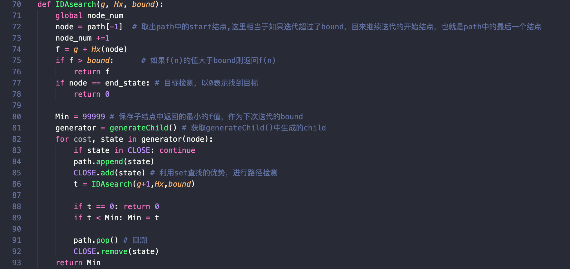
这部分是IDA*搜索算法的核心部分,在算法框架的基础上,加入了用set容器实现的CLOSE表,这与优化前不同的是,在优化之前,仍然是采用list进行路径检测,而之前提到过,从查找的角度来说,set的性能在大量数据的前提下是优于list的,因此在这里采用set进行判重,一方面起到了剪枝的作用,一方面能起到优化算法运行效率的作用。
2. A*搜索算法优化:
关键代码:
优化后:
A_star(start, Fx)
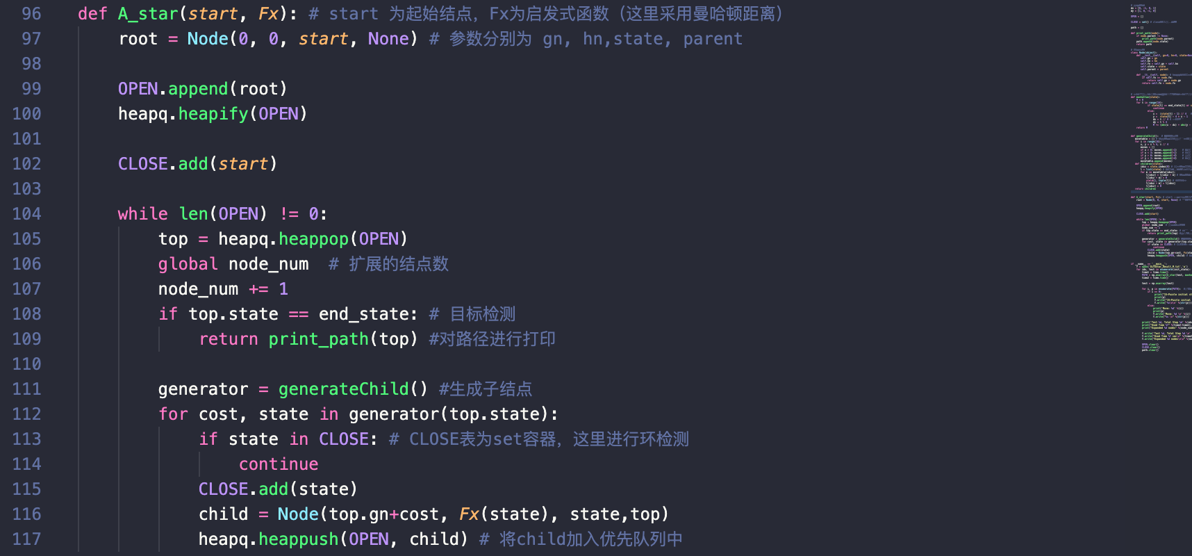
这里为A搜索算法的核心部分,环检测中以set作为状态存储的容器,这里的状态都以Tuple进行存储,因此可以直接加入set中;生成子结点的方式采用了与上方IDA同样的实现方式。
优化前:
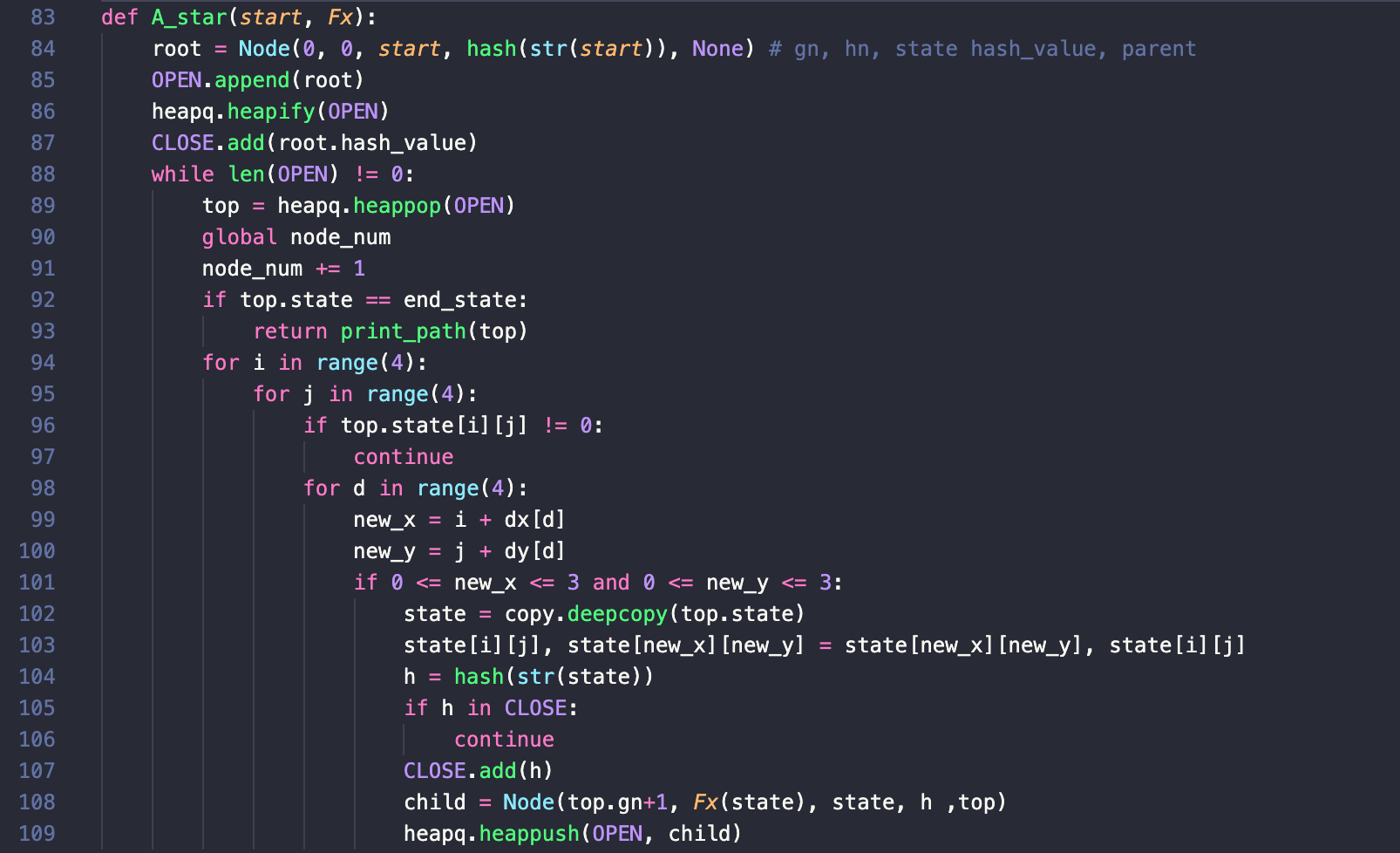
与优化前进行对比,由于采用了列表来存储状态,因此加入set中需要将其转换成字符串的形式,同时包含了繁琐的计算坐标移动的三重for循环。
3.实验结果:
下面,我们来看看在Example1-4上优化后的算法的结果如何:
Example1
A* 搜索算法运行结果:
Test 1, Total Step 40
Used Time 0.092726 sec
Expanded 3055 nodes
IDA* 搜索算法运行结果:
Test 1, Total Step 40
Used Time 0.261489 sec
Expanded 16334 nodes
Bound: 40
Example2
A* 搜索算法运行结果:
Test 2, Total Step 40
Used Time 0.039616 sec
Expanded 4240 nodes
IDA* 搜索算法运行结果:
Test 2, Total Step 40
Used Time 0.271453 sec
Expanded 30105 nodes
Bound: 40
Example3
A* 搜索算法运行结果:
Test 3, Total Step 40
Used Time 0.016239 sec
Expanded 4779 nodes
IDA* 搜索算法运行结果:
Test 3, Total Step 40
Used Time 0.098768 sec
Expanded 37683 nodes
Bound: 40
Example4
A* 搜索算法运行结果:
Test 4, Total Step 40
Used Time 0.483208 sec
Expanded 15259 nodes
IDA* 搜索算法运行结果:
Test 4, Total Step 40
Used Time 5.040609 sec
Expanded 256103 nodes
Bound: 40
总结:
测例Example1Example2Example3Example4优化前Used Time [A*| IDA*] (sec)0.30|1.190.13|0.520.06|0.240.98|18.74优化后Used Time[A* | IDA*] (sec)0.09|0.260.03|0.270.01|0.090.48|5.04Better [A* | IDA*]AAAA
优化前与优化后对比,IDA在运行时间上最高提高了4.5倍的性能,最少也有提升大约1.5倍,A在运行时间上最多提升6倍,最少提升了2倍。两者之中在这四个测例上仍然是A*算法占优。
补充:50步以上的测例
除了Example1-4上的测例以外,这里针对50步以上的测例四个测例,以优化前和优化后进行对比实验:
50步以上的测例
测例1 [[11, 3, 1, 7],[4, 6 ,8 ,2],[15 ,9 ,10, 13],[14, 12, 5 ,0]]

A* 搜索算法运行结果:
优化前
Test 1, Total Step 56
Used Time 2271.522129 sec
Expanded 18113640 nodes

优化后
Test 1, Total Step 56
Used Time 1077.335515 sec
Expanded 18116567 nodes
IDA* 搜索算法运行结果:
优化前:
时间过长

优化后:
Test 1, Total Step 56
Used Time 11228.500149 sec
Expanded 861726906 nodes
Bound: 56
测例2 [[14, 10, 6, 0],[4, 9 ,1 ,8],[2, 3, 5 ,11],[12, 13, 7 ,15]]

A* 搜索算法运行结果:
优化前:
Test 2, Total Step 53
Used Time 511.812972 sec
Expanded 22587975 nodes

优化后:
Test 2, Total Step 49
Used Time 54.638738 sec
Expanded 4438912 nodes
Bound: 49
IDA* 搜索算法运行结果:
优化前:
Test 2, Total Step 49
Used Time 493.416811 sec
Expanded 9890739 nodes
Bound: 49

优化后:
Test 2, Total Step 49
Used Time 54.638738 sec
Expanded 4438912 nodes
Bound: 49
测例3 [[0, 5, 15, 14],[7, 9, 6 ,13],[1, 2 ,12, 10],[8, 11, 4, 3]]

A* 搜索算法运行结果:
优化前:
Test 3, Total Step 64
Used Time 13271.092952 sec
Expanded 124070829 nodes

优化后:
Test 3, Total Step 64
Used Time 5099.071962 sec
Expanded 124434683 nodes
IDA* 搜索算法运行结果:
优化前:
时间过长

优化后:
时间过长
测例4 [[6 ,10, 3, 15],[14, 8, 7, 11],[5, 1, 0, 2],[13, 12, 9 ,4]]

A* 搜索算法运行结果:
优化前:
Test 4, Total Step 48
Used Time 170.719640 sec
Expanded 125820596 nodes

优化后:
Test 4, Total Step 48
Used Time 62.862862 sec
Expanded 126187137 nodes
IDA* 搜索算法运行结果:
优化前:
Test 4, Total Step 48
Used Time 1111.598261 sec
Expanded 20291684 nodes
Bound: 48

优化后:
Test 4, Total Step 48
Used Time 419.185472 sec
Expanded 34135093 nodes
Bound: 48
总结:
测例1234优化前Used Time [A*| IDA*] (sec)2271.5 |NaN511.8|493.413271.0|NaN170.7|1111.5优化后Used Time[A* | IDA*] (sec)1077.3|11228.554.6|54.65099.0| Nan62.8 |419.1Better [A* | IDA*]AIDAA*A
五、实现代码:
或者也可以Clone我的Github仓库并运行代码:Github代码链接
A*优化前:
#coding=utf-8import copy
import heapq
import numpy as np
import time

# 最终状态
end_state =[[1,2,3,4],[5,6,7,8],[9,10,11,12],[13,14,15,0]]
node_num  =0# 初始状态测例集
init_state =[[[1,15,7,10],[9,14,4,11],[8,5,0,6],[13,3,2,12]],#  [[1, 7, 8, 10],[6, 9, 15, 14], [13, 3, 0, 4], [11, 5, 12, 2]],#  [[5, 6, 4, 12], [11, 14, 9, 1], [0, 3, 8, 15], [10, 7, 2, 13]],#  [[14, 2, 8, 1], [7, 10, 4, 0], [6, 15, 11, 5], [9, 3, 13, 12]]# [[11, 3, 1, 7],[4, 6 ,8 ,2],[15 ,9 ,10, 13],[14, 12, 5 ,0]], #   [[14, 10, 6, 0],[4, 9 ,1 ,8],[2, 3, 5 ,11],[12, 13, 7 ,15]],# [[0, 5, 15, 14],[7, 9, 6 ,13],[1, 2 ,12, 10],[8, 11, 4, 3]],# [[6 ,10, 3, 15],[14, 8, 7, 11],[5, 1, 0, 2],[13, 12, 9 ,4]]#   [[1 , 3 ,10 , 4],[5 , 2  ,6 , 8], [14, 11 ,12 , 0], [7, 13,  9 ,15]]]# 方向数组
dx =[0,-1,0,1]
dy =[1,0,-1,0]

OPEN =[]

CLOSE =set()# close表,用于判重

path =[]defprint_path(node):if node.parent !=None:
        print_path(node.parent)
    path.append(node.state)return path

# 状态结点classNode(object):def__init__(self, gn=0, hn=0, state=None, hash_value=None, parent=None):
       self.gn = gn
       self.hn = hn
       self.fn = self.gn + self.hn
       self.state = state
       self.hash_value = hash_value
       self.parent = parent

    def__lt__(self, node):# heapq的比较函数if self.fn == node.fn:return self.gn > node.gn
        return self.fn < node.fn

defmanhattan(state):
    M =0for i inrange(4):for j inrange(4):if state[i][j]== end_state[i][j]or state[i][j]==0:continueelse:
                x =(state[i][j]-1)//4# 最终坐标
                y = state[i][j]-4* x -1
                M +=(abs(x - i)+abs(y - j))return M

defmisplaced(state):sum=0for i inrange(4):for j inrange(4):if state[i][j]==0:continueif state[i][j]!= end_state[i][j]:sum+=1returnsumdefA_star(start, Fx):
    root = Node(0,0, start,hash(str(start)),None)# gn, hn, state hash_value, parent
    OPEN.append(root)
    heapq.heapify(OPEN)
    CLOSE.add(root.hash_value)whilelen(OPEN)!=0:
        top = heapq.heappop(OPEN)global node_num
        node_num +=1if top.state == end_state:return print_path(top)for i inrange(4):for j inrange(4):if top.state[i][j]!=0:continuefor d inrange(4):
                    new_x = i + dx[d]
                    new_y = j + dy[d]if0<= new_x <=3and0<= new_y <=3:
                        state = copy.deepcopy(top.state)
                        state[i][j], state[new_x][new_y]= state[new_x][new_y], state[i][j]
                        h =hash(str(state))if h in CLOSE:continue
                        CLOSE.add(h)
                        child = Node(top.gn+1, Fx(state), state, h ,top)
                        heapq.heappush(OPEN, child)if __name__ =='__main__':
    f =open('AStar_result.txt','w')for idx, test inenumerate(init_state):
        time1 = time.time()
        PATH = np.asarray(A_star(test, manhattan))
        time2 = time.time()

        test = np.asarray(test)for i, p inenumerate(PATH):#路径打印if i ==0:print("15-Puzzle initial state:")print(p)
                 f.write("15-Puzzle initial state:\n")
                 f.write('%s\n\n'%(str(p)))else:print('Move: %d'%(i))print(p)
                f.write('Move: %d \n'%(i))
                f.write("%s \n"%(str(p)))print('Test %d, Total Step %d'%(idx+1,len(path)-1))print("Used Time %f"%(time2-time1),"sec")print("Expanded %d nodes"%(node_num))

        f.write('Test %d, Total Step %d \n'%(idx+1,len(path)-1))
        f.write("Used Time %f sec\n"%(time2-time1))
        f.write("Expanded %d nodes\n\n"%(node_num))

        OPEN.clear()
        CLOSE.clear()
        path.clear()
A*优化后:
#coding=utf-8import copy
import heapq
import numpy as np
import time

# 最终状态
node_num  =0
end_state =(1,2,3,4,5,6,7,8,9,10,11,12,13,14,15,0)# 初始状态测例集
init_state =[(1,15,7,10,9,14,4,11,8,5,0,6,13,3,2,12),#(1, 7, 8, 10,6, 9, 15, 14, 13, 3, 0, 4, 11, 5, 12, 2),#(5, 6, 4, 12, 11, 14, 9, 1, 0, 3, 8, 15, 10, 7, 2, 13),#(14, 2, 8, 1, 7, 10, 4, 0, 6, 15, 11, 5, 9, 3, 13, 12),#(11, 3, 1, 7,4, 6 ,8 ,2,15 ,9 ,10, 13,14, 12, 5 ,0), #(14, 10, 6, 0,4, 9 ,1 ,8,2, 3, 5 ,11,12, 13, 7 ,15),#(0, 5, 15, 14,7, 9, 6 ,13,1, 2 ,12, 10,8, 11, 4, 3),#  (6 ,10, 3, 15,14, 8, 7, 11,5, 1, 0, 2,13, 12, 9 ,4)]# 方向数组
dx =[0,-1,0,1]
dy =[1,0,-1,0]

OPEN =[]

CLOSE =set()# close表,用于判重

path =[]defprint_path(node):if node.parent !=None:
        print_path(node.parent)
    path.append(node.state)return path

# 状态结点classNode(object):def__init__(self, gn=0, hn=0, state=None, parent=None):
       self.gn = gn
       self.hn = hn
       self.fn = self.gn + self.hn
       self.state = state
       self.parent = parent

    def__lt__(self, node):# heapq的比较函数if self.fn == node.fn:return self.gn > node.gn
        return self.fn < node.fn

# 曼哈顿距离(注意:不需要计算‘0’的曼哈顿值,否则不满足Admittable)defmanhattan(state):
    M =0for t inrange(16):if state[t]== end_state[t]or state[t]==0:continueelse:
                x =(state[t]-1)//4# 最终坐标
                y =  state[t]-4* x -1
                dx = t //4# 实际坐标
                dy = t %4
                M +=(abs(x - dx)+abs(y - dy))return M

defgenerateChild():# 生成子结点
   movetable =[]# 针对数码矩阵上每一个可能的位置,生成其能够移动的方向列表for i inrange(16):
       x, y = i %4, i //4
       moves =[]if x >0: moves.append(-1)# 左移if x <3: moves.append(+1)# 右移if y >0: moves.append(-4)# 上移if y <3: moves.append(+4)# 下移
       movetable.append(moves)defchildren(state):
       idxz = state.index(0)# 寻找数码矩阵上0的坐标
       l =list(state)# 将元组转换成list,方便进行元素修改for m in movetable[idxz]:
           l[idxz]= l[idxz + m]# 数码交换位置
           l[idxz + m]=0yield(1,tuple(l))# 临时返回
           l[idxz + m]= l[idxz]
           l[idxz]=0return children

defA_star(start, Fx):# start 为起始结点,Fx为启发式函数(这里采用曼哈顿距离)
    root = Node(0,0, start,None)# 参数分别为 gn, hn,state, parent

    OPEN.append(root)
    heapq.heapify(OPEN)

    CLOSE.add(start)whilelen(OPEN)!=0:
        top = heapq.heappop(OPEN)global node_num  # 扩展的结点数
        node_num +=1if top.state == end_state:# 目标检测return print_path(top)#对路径进行打印

        generator = generateChild()#生成子结点for cost, state in generator(top.state):if state in CLOSE:# CLOSE表为set容器,这里进行环检测continue
            CLOSE.add(state)
            child = Node(top.gn+cost, Fx(state), state,top)
            heapq.heappush(OPEN, child)# 将child加入优先队列中if __name__ =='__main__':
    f =open('AStar_Result_M.txt','w')for idx, test inenumerate(init_state):
        time1 = time.time()
        PATH = np.asarray(A_star(test, manhattan))
        time2 = time.time()

        test = np.asarray(test)for i, p inenumerate(PATH):#路径打印if i ==0:print("15-Puzzle initial state:")print(p)
                 f.write("15-Puzzle initial state:\n")
                 f.write('%s\n\n'%(str(p)))else:print('Move: %d'%(i))print(p)
                f.write('Move: %d \n'%(i))
                f.write("%s \n"%(str(p)))print('Test %d, Total Step %d'%(idx+1,len(path)-1))print("Used Time %f"%(time2-time1),"sec")print("Expanded %d nodes"%(node_num))

        f.write('Test %d, Total Step %d \n'%(idx+1,len(path)-1))
        f.write("Used Time %f sec\n"%(time2-time1))
        f.write("Expanded %d nodes\n\n"%(node_num))

        OPEN.clear()
        CLOSE.clear()
        path.clear()
IDA*优化前:
import numpy as np
import time
import copy
# 最终状态
end_state =[[1,2,3,4],[5,6,7,8],[9,10,11,12],[13,14,15,0]]
node_num =0# 初始状态测例集
init_state =[[[1,15,7,10],[9,14,4,11],[8,5,0,6],[13,3,2,12]],#  [[1, 7, 8, 10],[6, 9, 15, 14], [13, 3, 0, 4], [11, 5, 12, 2]],# [[5, 6, 4, 12], [11, 14, 9, 1], [0, 3, 8, 15], [10, 7, 2, 13]],#  [[14, 2, 8, 1], [7, 10, 4, 0], [6, 15, 11, 5], [9, 3, 13, 12]]#  [[11, 3, 1, 7],[4, 6 ,8 ,2],[15 ,9 ,10, 13],[14, 12, 5 ,0]],  # [[14, 10, 6, 0],[4, 9 ,1 ,8],[2, 3, 5 ,11],[12, 13, 7 ,15]],# [[0, 5, 15, 14],[7, 9, 6 ,13],[1, 2 ,12, 10],[8, 11, 4, 3]],# [[6 ,10, 3, 15],[14, 8, 7, 11],[5, 1, 0, 2],[13, 12, 9 ,4]]]
CLOSE ={}# 方向数组
dx =[0,-1,0,1]
dy =[1,0,-1,0]defis_goal(node):
    index =1for row in node:for col in row:if(index != col):break
            index +=1return index ==16# 曼哈顿距离(注意:不需要计算‘0’的曼哈顿值,否则不满足Admittable)defmanhattan(state):
    M =0for i inrange(4):for j inrange(4):if state[i][j]== end_state[i][j]or state[i][j]==0:continue# if state[i][j] == 0:#     x, y = 3, 3 else:
                x =int((state[i][j]-1)/4)# 最终坐标
                y =  state[i][j]-4* x -1
                M +=(abs(x - i)+abs(y - j))return M

defmisplaced(state):sum=0for i inrange(4):for j inrange(4):if state[i][j]==0:continueif state[i][j]!= end_state[i][j]:sum+=1returnsumdefgenerateChild(state, Hx):# 生成子结点
    child =[]# 用于保存生成的子结点for i inrange(4):for j inrange(4):if state[i][j]!=0:continuefor d inrange(4):
                    new_x = i + dx[d]
                    new_y = j + dy[d]if0<= new_x <=3and0<= new_y <=3:
                        new_state = copy.deepcopy(state)
                        new_state[i][j], new_state[new_x][new_y]= new_state[new_x][new_y], new_state[i][j]
                        child.append(new_state)returnsorted(child, key=lambda x: Hx(x))# 将子结点进行排序,以H(n)递增排序defIDAsearch(path, g, Hx, bound):# global node_num
    node = path[-1]# 取出path中的start结点,这里相当于如果迭代超过了bound,回来继续迭代的开始结点,也就是path中的最后一个结点
    node_num +=1#  print(node_num)
    f = g + Hx(node)if f > bound:# 如果f(n)的值大于bound则返回f(n)return f
    if node == end_state:# 目标检测,以0表示找到目标return0

    Min =99999
    CLOSE[str(node)]= g
   # print(CLOSE)for c in generateChild(node, Hx):# 遍历该结点所扩展的孩子结点#import pdb; pdb.set_trace()# if c not in path:  # 路径检测#     if str(c) in CLOSE: # 环检测#         f = g + 1 #         fp = CLOSE.get(str(c))#         if fp > f:#             print('in',c,CLOSE.get(str(c)) )#             CLOSE[str(c)] = f#         else: #             continue
            path.append(c)
            t = IDAsearch(path, g+1, Hx, bound)if t ==0:# 如果得到的返回值为0,表示找到目标,迭代结束return0if t < Min:# 如果返回值不是0,说明f>bound,这时对Min进行更新,取值最小的返回值作为Min
                Min = t
            path.pop()# 深搜回溯return Min

defIDAstar(start, Hx):
    bound = Hx(start)# IDA*迭代限制
    path =[start]# 路径集合, 视为栈
    CLOSE[str(start)]=0#CLOSE.add(hash(str(start)))while(True):
        ans = IDAsearch(path,0, Hx,bound)# path, g, Hx, boundif(ans ==0):return(path,bound)if ans ==-1:returnNone
        bound = ans # 此处对bound进行更新if __name__ =='__main__':
    f =open('IDAStar_Difresult.txt','w')for idx, test inenumerate(init_state):
        time1 = time.time()
        PATH,BOUND = IDAstar(test, misplaced)
        time2 = time.time()
        PATH = np.asarray(PATH)

        test = np.asarray(test)for i, p inenumerate(PATH):#路径打印if i ==0:print("15-Puzzle initial state:")
                 f.write("15-Puzzle initial state:\n")

                 p = np.asarray(p)print(p)
                 f.write('%s\n\n'%(str(p)))else:print('Move: %d'%(i))

                f.write('Move: %d \n'%(i))
                p = np.asarray(p)print(p)
                f.write("%s \n"%(str(p)))print('Test %d, Total Step %d'%(idx+1,len(PATH)-1))print("Used Time %f"%(time2-time1),"sec")print("Expanded %d nodes"%(node_num))print("Bound: %d"%(BOUND))

        f.write('Test %d, Total Step %d \n'%(idx+1,len(PATH)-1))
        f.write("Used Time %f sec\n"%(time2-time1))
        f.write("Expanded %d nodes\n"%(node_num))
        f.write("Bound: %d\n\n"%(BOUND))
IDA*优化后:
import numpy as np
import time
import copy
# 最终状态
end_state =(1,2,3,4,5,6,7,8,9,10,11,12,13,14,15,0)
node_num =0# 初始状态测例集
init_state =[(1,15,7,10,9,14,4,11,8,5,0,6,13,3,2,12),# (1, 7, 8, 10,6, 9, 15, 14, 13, 3, 0, 4, 11, 5, 12, 2),# (5, 6, 4, 12, 11, 14, 9, 1, 0, 3, 8, 15, 10, 7, 2, 13),# (14, 2, 8, 1, 7, 10, 4, 0, 6, 15, 11, 5, 9, 3, 13, 12),#  (11, 3, 1, 7,4, 6 ,8 ,2,15 ,9 ,10, 13,14, 12, 5 ,0),  # (14, 10, 6, 0,4, 9 ,1 ,8,2, 3, 5 ,11,12, 13, 7 ,15),(0,5,15,14,7,9,6,13,1,2,12,10,8,11,4,3),#(6 ,10, 3, 15,14, 8, 7, 11,5, 1, 0, 2,13, 12, 9 ,4)]

CLOSE =set()#  用于判重
path =[]# 方向数组
dx =[0,-1,0,1]
dy =[1,0,-1,0]# 曼哈顿距离(注意:不需要计算‘0’的曼哈顿值,否则不满足Admittable)defmanhattan(state):
    M =0for t inrange(16):if state[t]== end_state[t]or state[t]==0:continueelse:
                x =(state[t]-1)//4# 最终坐标
                y =  state[t]-4* x -1
                dx = t //4# 实际坐标
                dy = t %4
                M +=(abs(x - dx)+abs(y - dy))return M

defgenerateChild():# 生成子结点
   movetable =[]# 针对数码矩阵上每一个可能的位置,生成其能够移动的方向列表for i inrange(16):
       x, y = i %4, i //4
       moves =[]if x >0: moves.append(-1)# 左移if x <3: moves.append(+1)# 右移if y >0: moves.append(-4)# 上移if y <3: moves.append(+4)# 下移
       movetable.append(moves)defchildren(state):
       idxz = state.index(0)# 寻找数码矩阵上0的坐标
       l =list(state)# 将元组转换成list,方便进行元素修改for m in movetable[idxz]:
           l[idxz]= l[idxz + m]# 数码交换位置
           l[idxz + m]=0yield(1,tuple(l))# 临时返回
           l[idxz + m]= l[idxz]
           l[idxz]=0return children

defIDAsearch(g, Hx, bound):global node_num
    node = path[-1]# 取出path中的start结点,这里相当于如果迭代超过了bound,回来继续迭代的开始结点,也就是path中的最后一个结点
    node_num +=1
    f = g + Hx(node)if f > bound:# 如果f(n)的值大于bound则返回f(n)return f
    if node == end_state:# 目标检测,以0表示找到目标return0

    Min =99999# 保存子结点中返回的最小的f值,作为下次迭代的bound
    generator = generateChild()# 获取generateChild()中生成的childfor cost, state in generator(node):if state in CLOSE:continue
        path.append(state)
        CLOSE.add(state)# 利用set查找的优势,进行路径检测
        t = IDAsearch(g+1,Hx,bound)if t ==0:return0if t < Min: Min = t

        path.pop()# 回溯
        CLOSE.remove(state)return Min


defIDAstar(start, Hx):global CLOSE
    global path
    bound = Hx(start)# IDA*迭代限制
    path =[start]# 路径集合, 视为栈
    CLOSE ={start}while(True):
        ans = IDAsearch(0, Hx,bound)# path, g, Hx, boundif(ans ==0):return(path,bound)if ans ==-1:returnNone
        bound = ans # 此处对bound进行更新if __name__ =='__main__':
    f =open('IDAStar_result.txt','w')for idx, test inenumerate(init_state):
        time1 = time.time()
        PATH,BOUND = IDAstar(test, manhattan)
        time2 = time.time()
        PATH = np.asarray(PATH)

        test = np.asarray(test)for i, p inenumerate(PATH):#路径打印if i ==0:print("15-Puzzle initial state:")
                 f.write("15-Puzzle initial state:\n")

                 p = np.asarray(p)print(p)
                 f.write('%s\n\n'%(str(p)))else:print('Move: %d'%(i))

                f.write('Move: %d \n'%(i))
                p = np.asarray(p)print(p)
                f.write("%s \n"%(str(p)))print('Test %d, Total Step %d'%(idx+1,len(PATH)-1))print("Used Time %f"%(time2-time1),"sec")print("Expanded %d nodes"%(node_num))print("Bound: %d"%(BOUND))

        f.write('Test %d, Total Step %d \n'%(idx+1,len(PATH)-1))
        f.write("Used Time %f sec\n"%(time2-time1))
        f.write("Expanded %d nodes\n"%(node_num))
        f.write("Bound: %d\n\n"%(BOUND))
版权归原作者 Maxwell-Wong 所有, 如有侵权,请联系我们删除。