【代码解读】超详细，YOLOV5之build_targets函数解读。

文章目录

build_targets作用

build_targets函数用于网络训练时计算loss所需要的目标框，即正样本。

注意

1. 与yolov3/yolov4不同，yolv5支持跨网格预测。即每一个bbox，正对于任何一个输出层，都可能有anchor与之匹配。
2. 该函数输出的正样本框比传入的GT数目要多。
3. 当前解读版本为6.1

可视化结果

• TODO

过程

1. 首先通过bbox与当前层anchor做一遍过滤。对于任何一层计算当前bbox与当前层anchor的匹配程度，不采用IoU，而采用shape比例。如果anchor与bbox的宽高比差距大于4，则认为不匹配，保留下匹配的bbox。

 r = t[...,4:6]/ anchors[:,None]# wh ratio
 j = torch.max(r,1/ r).max(2)[0]< self.hyp['anchor_t']# compare# j = wh_iou(anchors, t[:, 4:6]) > model.hyp['iou_t']  # iou(3,n)=wh_iou(anchors(3,2), gwh(n,2))
 t = t[j]# filter

1. 最后根据留下的bbox，在上下左右四个网格四个方向扩增采样。

 gxy = t[:,2:4]# grid xy
 gxi = gain[[2,3]]- gxy  # inverse
 j, k =((gxy %1< g)&(gxy >1)).T
 l, m =((gxi %1< g)&(gxi >1)).T
 j = torch.stack((torch.ones_like(j), j, k, l, m))
 t = t.repeat((5,1,1))[j]

详细代码解读

准备

defbuild_targets(self, p, targets):

P是网络预测的输出。

p的shape为

:(batch_size,anchor_num,grid_cell,grid_cell,xywh+obj_confidence+classes_num)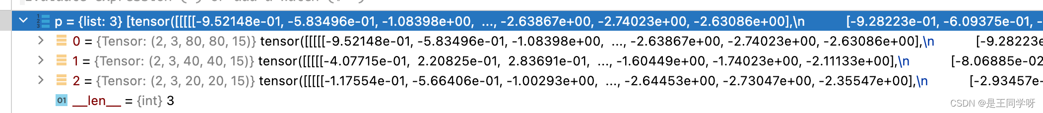

P[0]的shape

P[1]的shape

P[2]的shape

targets是经过数据增强(mosaic等)后总的bbox。

targets的shape为

：[num_obj, 6] , that number 6 means -> (img_index, obj_index, x, y, w, h)

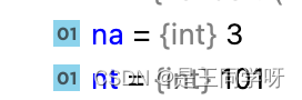
na, nt = self.na, targets.shape[0]# number of anchors, targets

tcls, tbox, indices, anch =[],[],[],[]

tcls：用来存储类别。
tbox：用来存储bbox
indices：用来存储第几张图片，当前层的第几个anchor，以及当前层grid的下标。

gain = torch.ones(7, device=self.device)# normalized to gridspace gain

初始化为1，用来还原bbox为当前层的尺度大小。

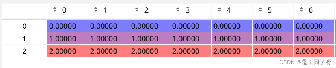
 ai = torch.arange(na, device=self.device).float().view(na,1).repeat(1, nt)# same as .repeat_interleave(nt)

扩充anchor数量和当前bbox一样多。
ai是anchor的下标

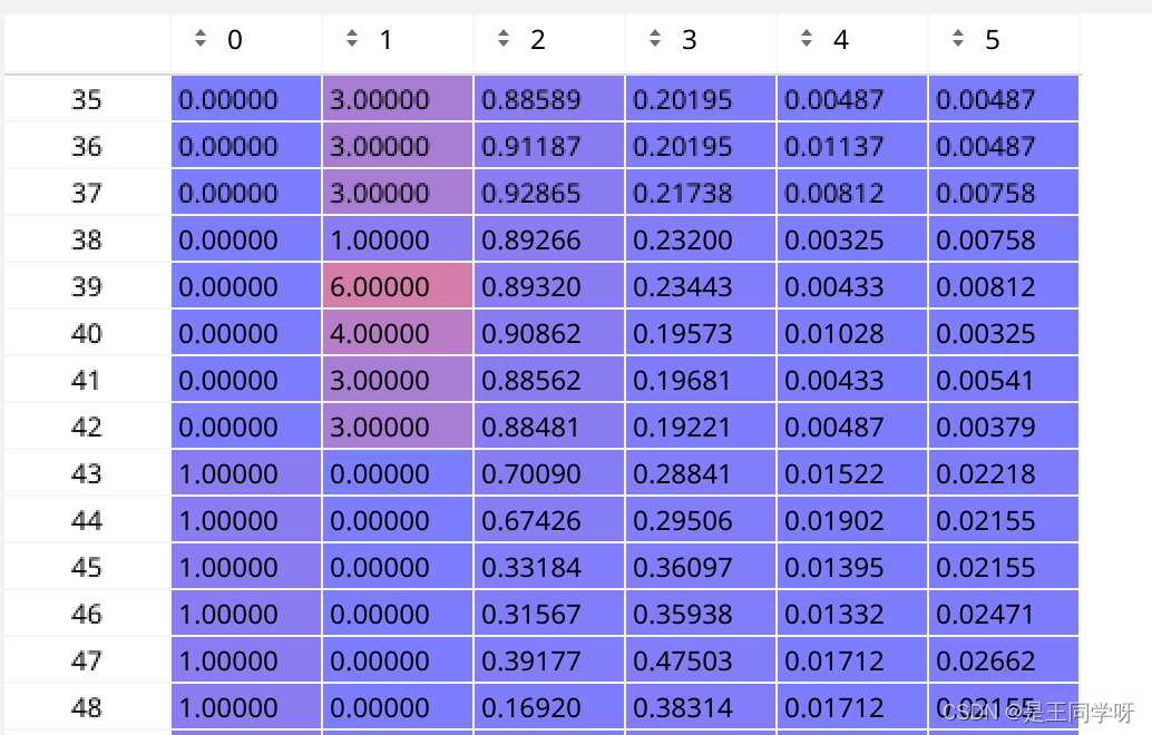
targets = torch.cat((targets.repeat(na,1,1), ai[...,None]),2)# append anchor indices

targets的shape变为(3,101,7)。

targets[0]

对应第一个anchor对应的(image_id, cls, center_x,center_y, w, h,第一个anchor)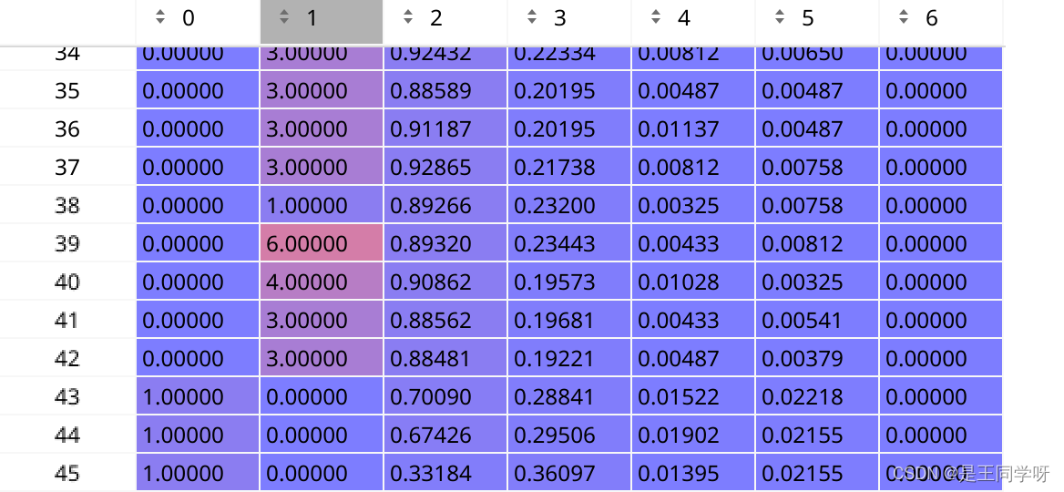

targets[1]

对应第一个anchor对应的(image_id, cls, center_x,center_y, w, h,第二个anchor)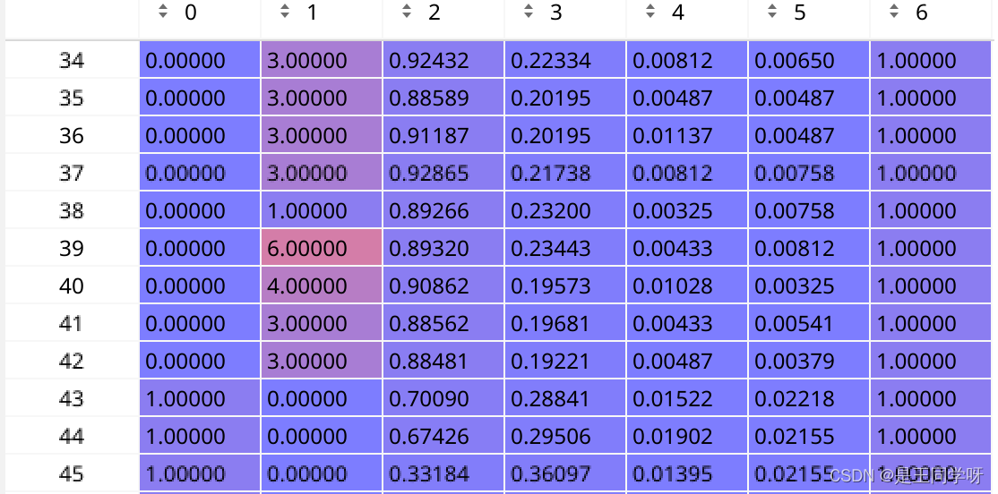

targets[2]

对应第一个anchor对应的(image_id, cls, center_x,center_y, w, h,第三个anchor)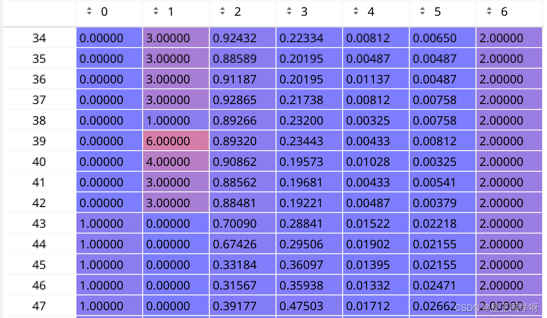

# 预定义的偏移量
 g =0.5# bias
 off = torch.tensor([[0,0],[1,0],[0,1],[-1,0],[0,-1],# j,k,l,m# [1, 1], [1, -1], [-1, 1], [-1, -1],  # jk,jm,lk,lm],
     device=self.device).float()* g  # offsets

for i inrange(self.nl):# 枚举每一层

anchors = self.anchors[i]# 当前层anchor

self.anchors

self.anchors[0]

得到第一层归一化后的anchor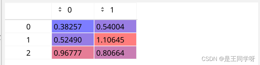

乘8得到的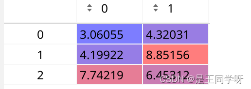

self.anchors[1]

得到第二层归一化后的anchor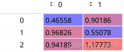

乘16得到的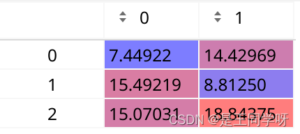

self.anchors[2]

得到第三层归一化后的anchor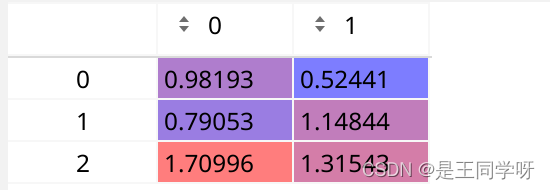

乘以32得到的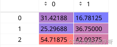

gain[2:6]= torch.tensor(p[i].shape)[[3, 2, 3, 2]]# xyxy gain

生成一个当前层的方格大小。
如果i=0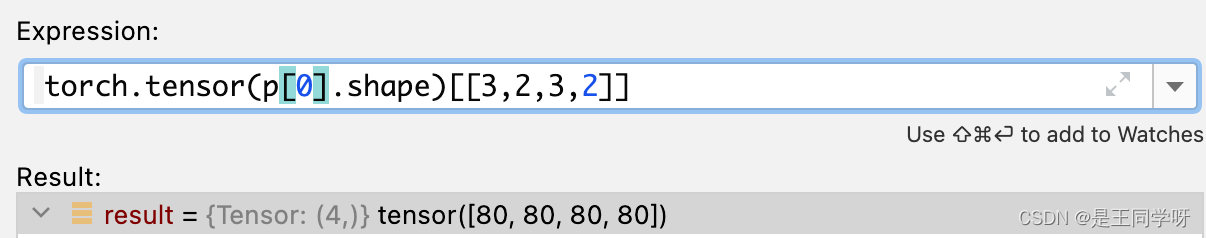

如果i=1，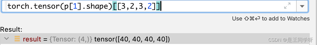

如果i=2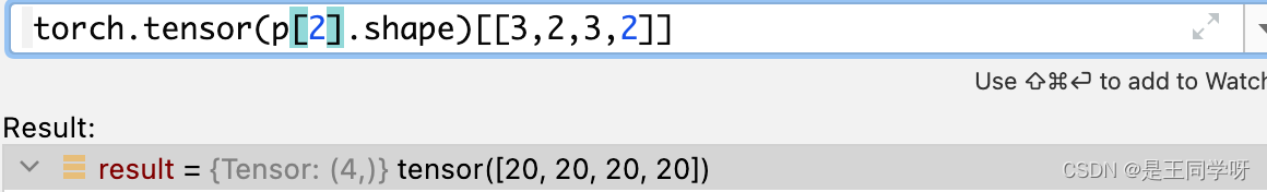

t = targets * gain

将targets的大小映射到当前层，第六列是当前层的第几个anchor,第0列是位于哪张图片，第1列代表的是类别，2-5列是目标在当前层x,y,w,h。
下采样八倍的层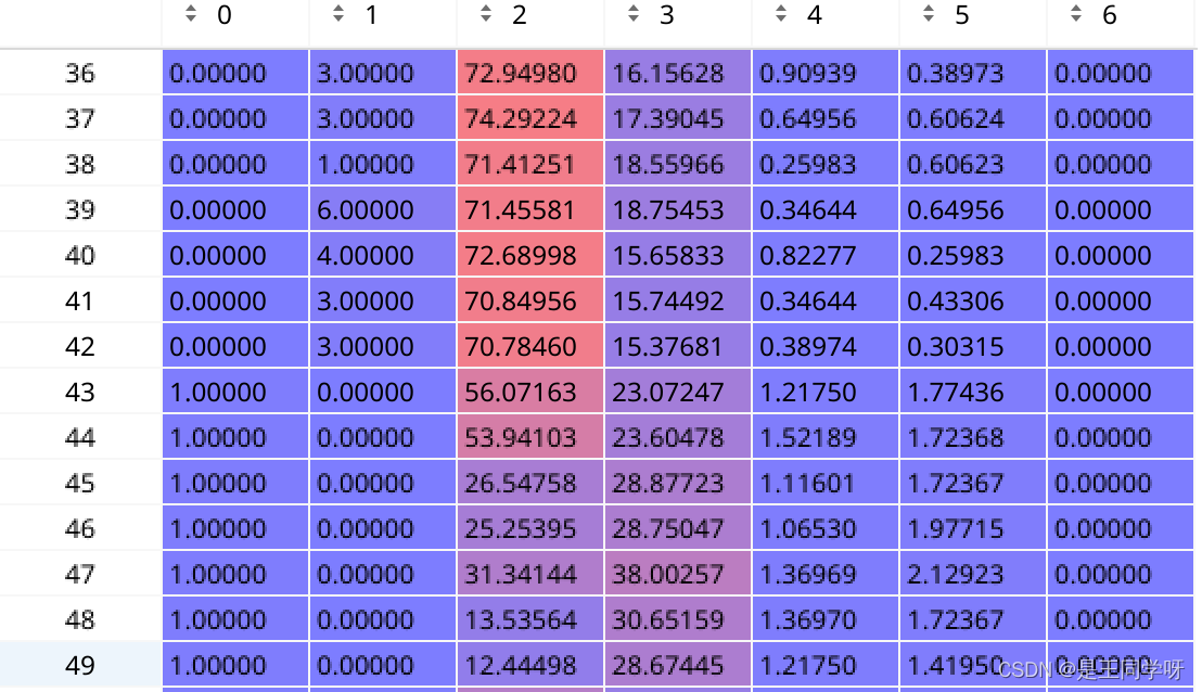

第一遍筛选

if nt:# 如果存在目标

r = t[..., 4:6] / anchors[:, None]

r是指bbox与当前层三个anchor的高宽的比值。

r[0]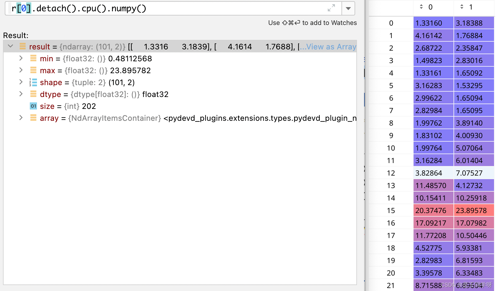

r[1]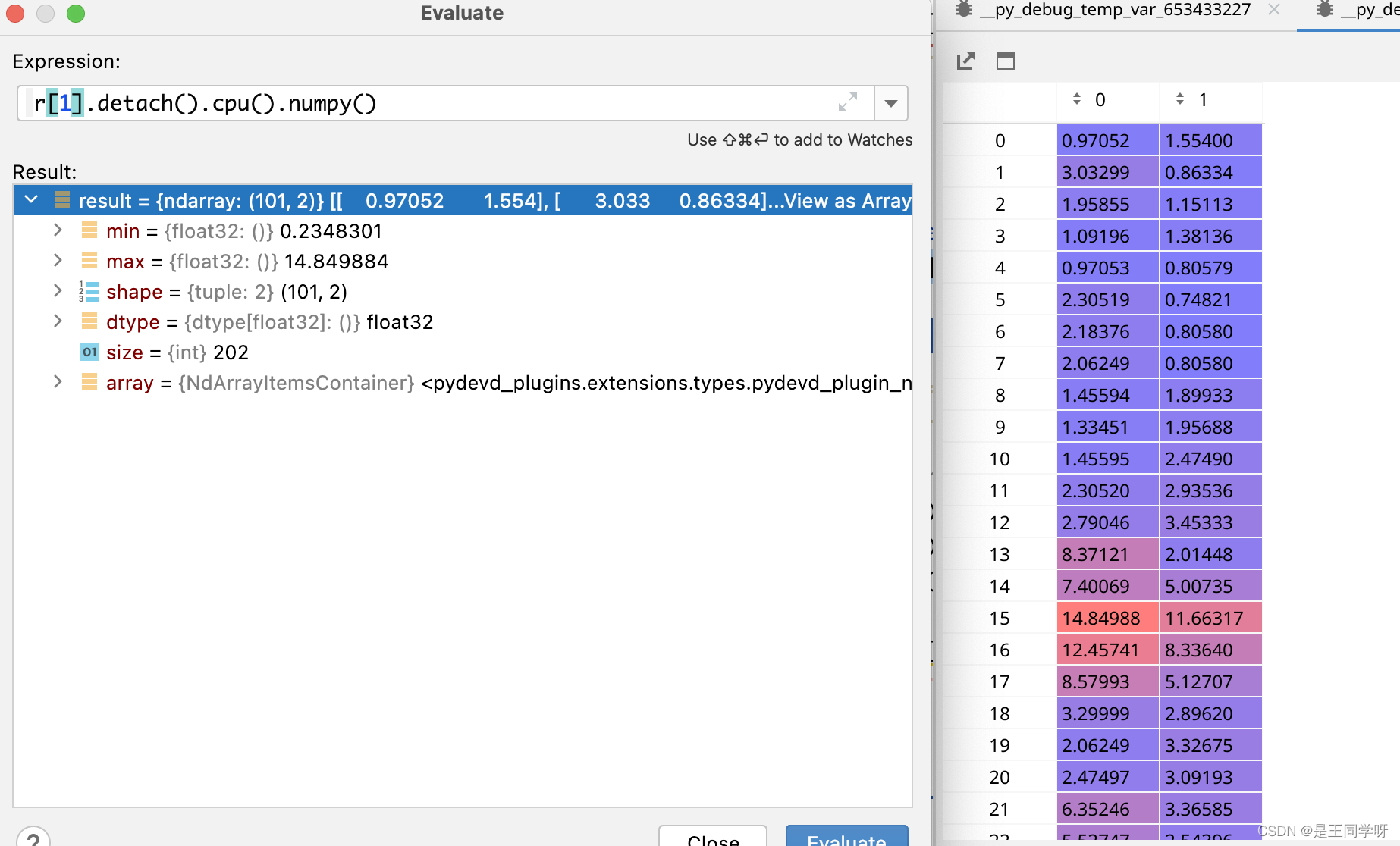

r[2]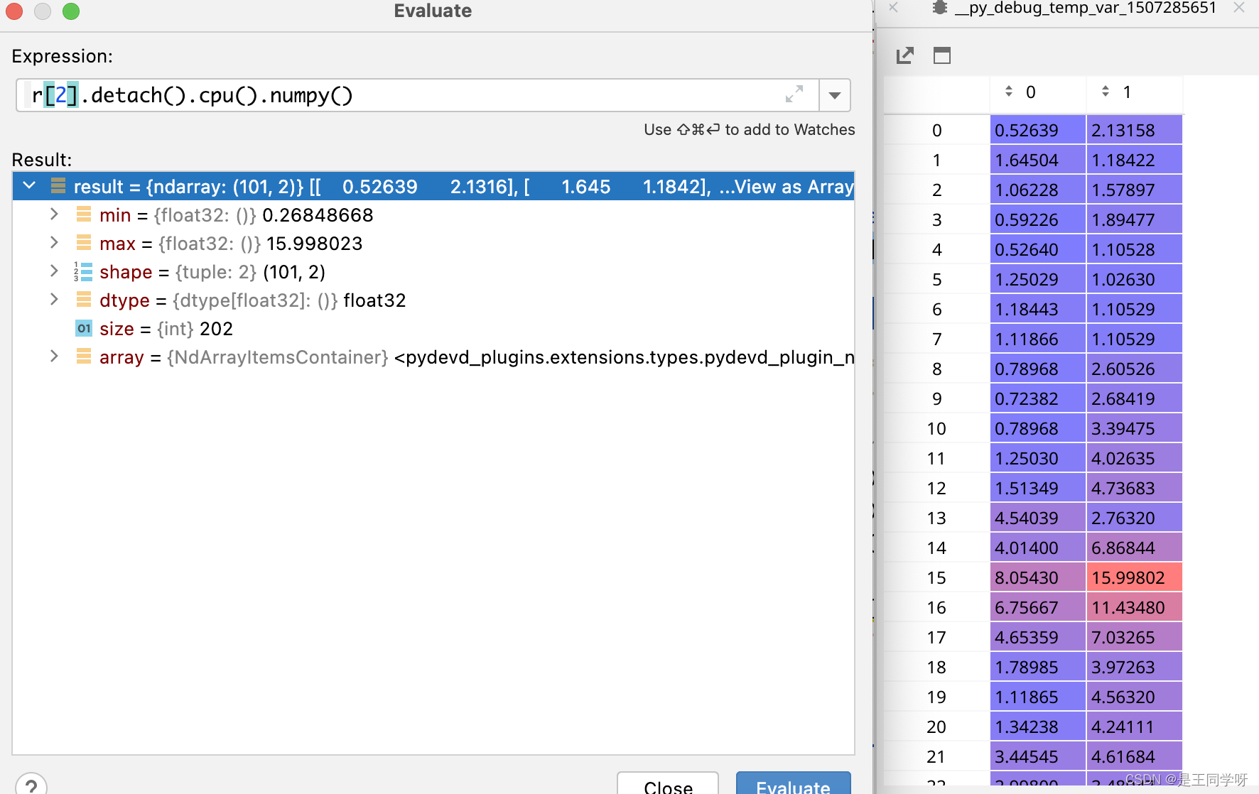

j = torch.max(r, 1 / r).max(2)[0]< self.hyp['anchor_t']# compare

torch.max(r, 1 / r).max(2)[0]

为什么是

[0]

不是

[1]

.[0]代表的是value,[1]代表的index。

torch.max(r, 1 / r).max(2)[1]

torch.max(r, 1 / r).max(1)[0]

按行获取最大值。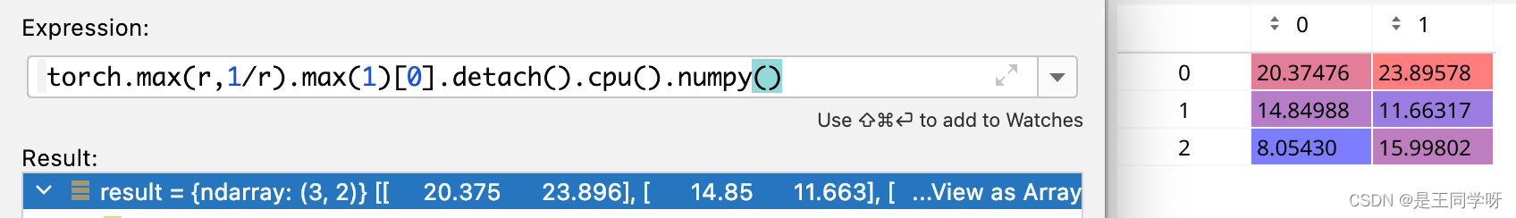

torch.max(r, 1 / r).max(1)[1]

按行获取最大值，返回索引。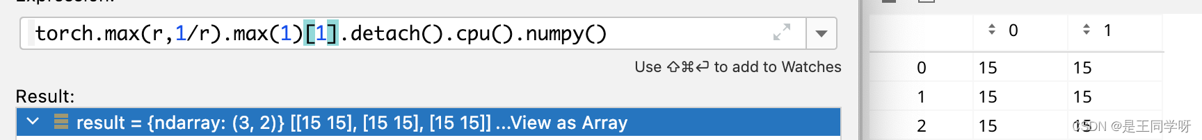

t = t[j]# filter

经过过滤后，全部汇总到来了一起。按照第六列anchor的顺序排列。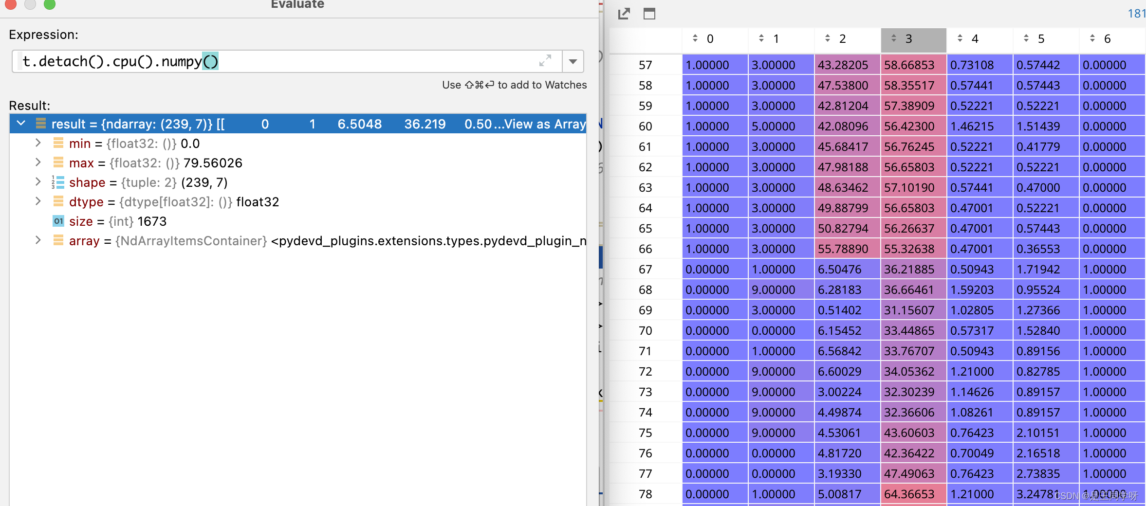

扩增正样本

接下来是扩增正样本

gxy = t[:,2:4]# grid xy  # 获取x,y
gxi = gain[[2,3]]- gxy  # inverse

假设最后的特征图大小是8x8,有a-h8个目标边框如下。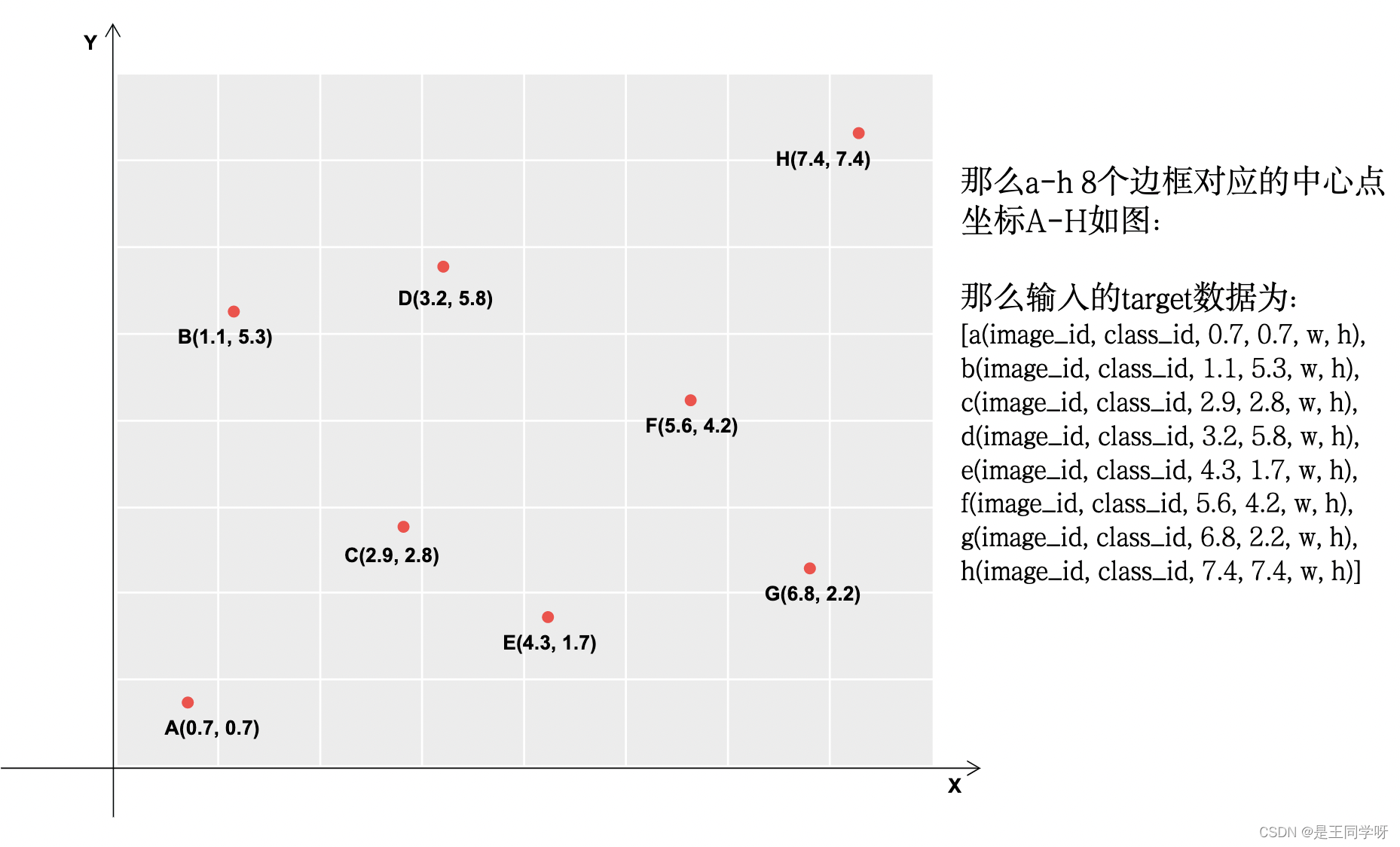

下图中深灰色的表示满足条件的。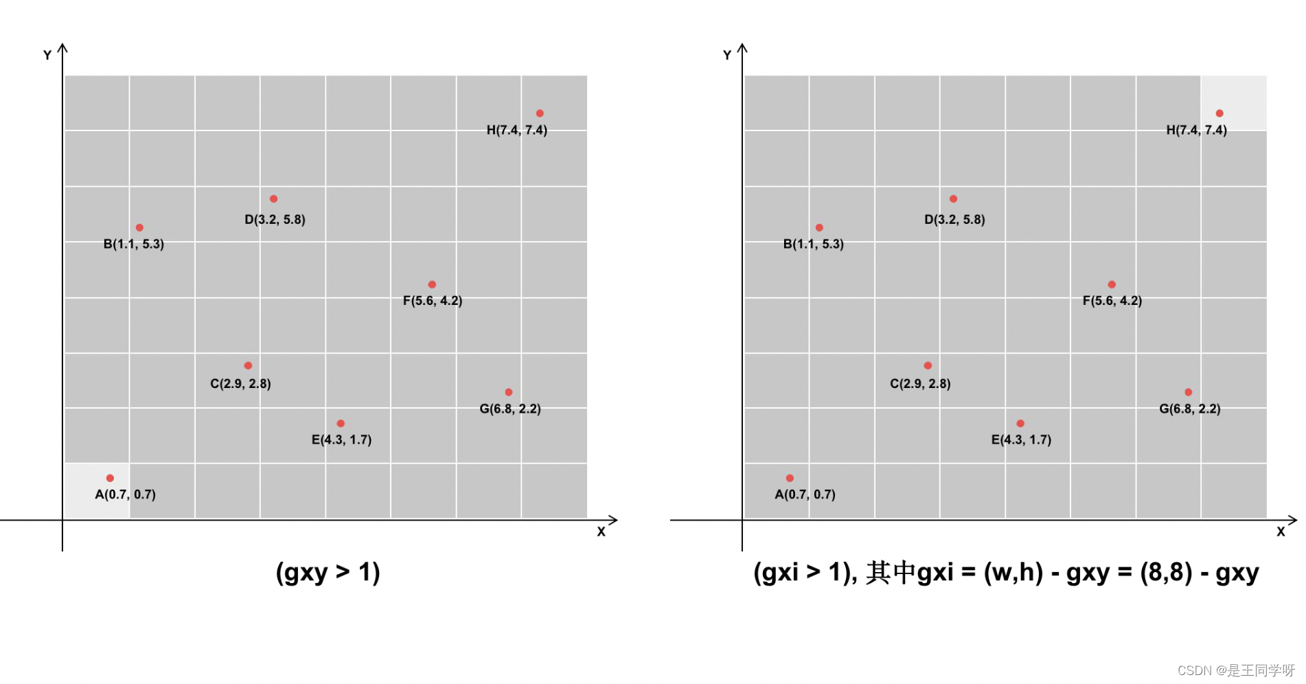

j, k =((gxy %1< g)&(gxy >1)).T
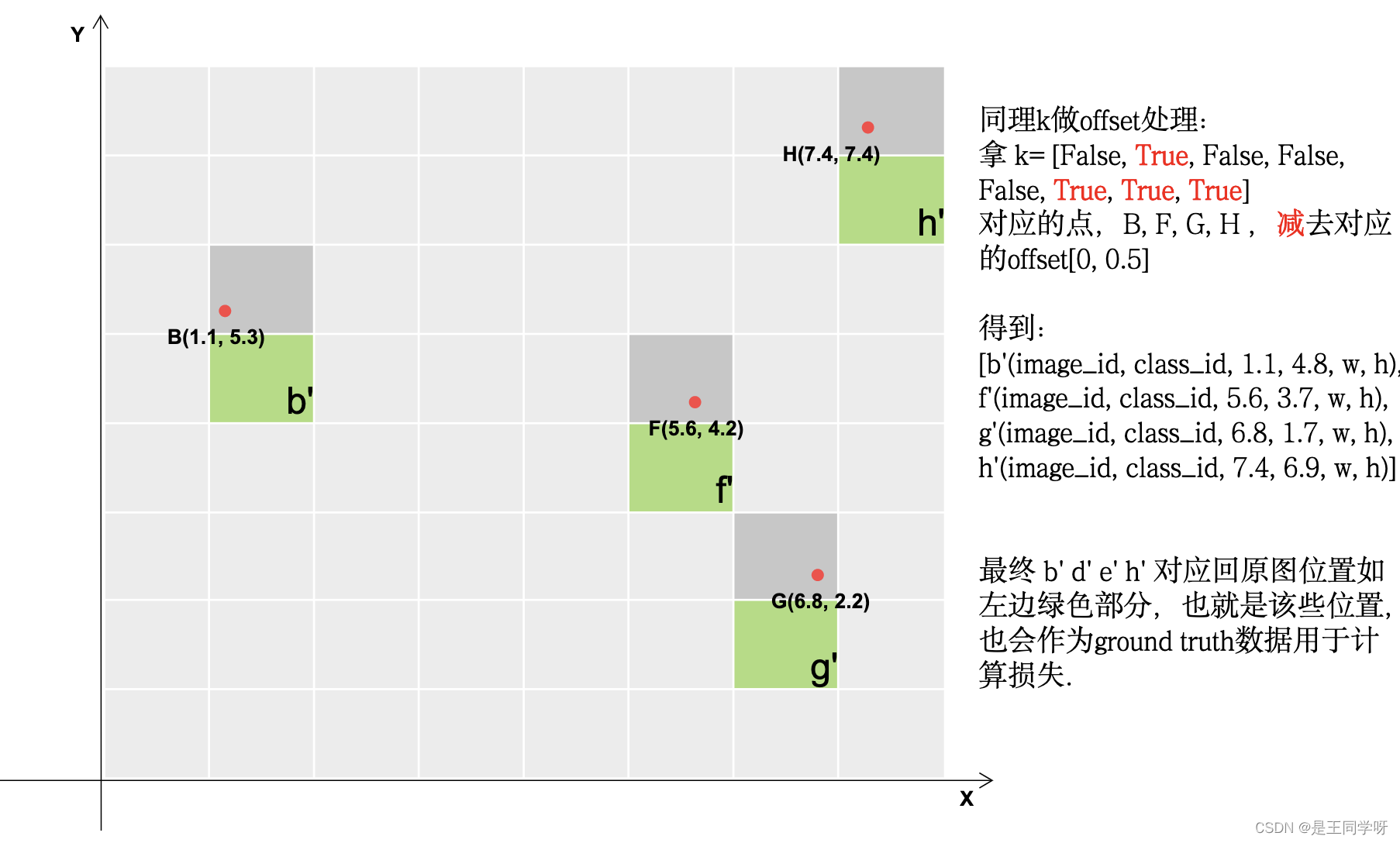
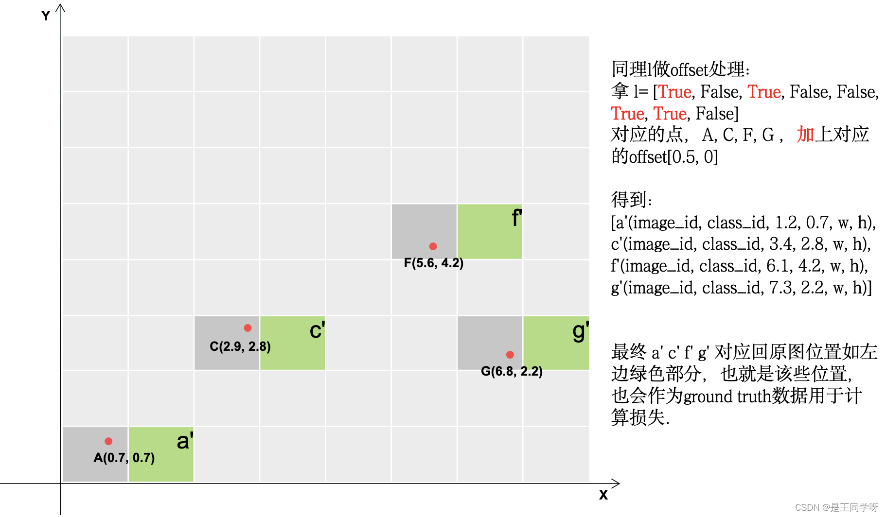
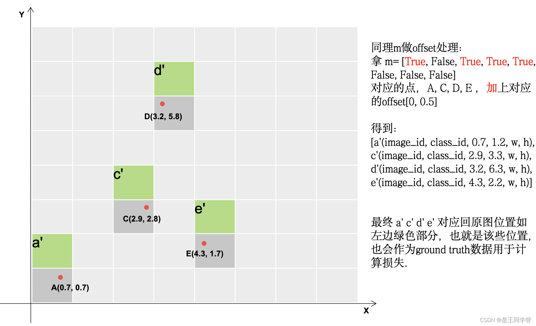
l, m =((gxi %1< g)&(gxi >1)).T

gxy % 1 < g

和

gxi % 1 < g

包含两个方向，x和y方向。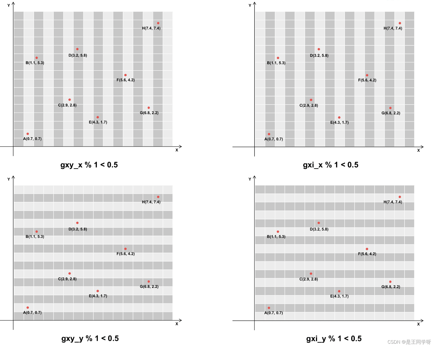

((gxy %1< g)&(gxy >1))#条件合并得到下图

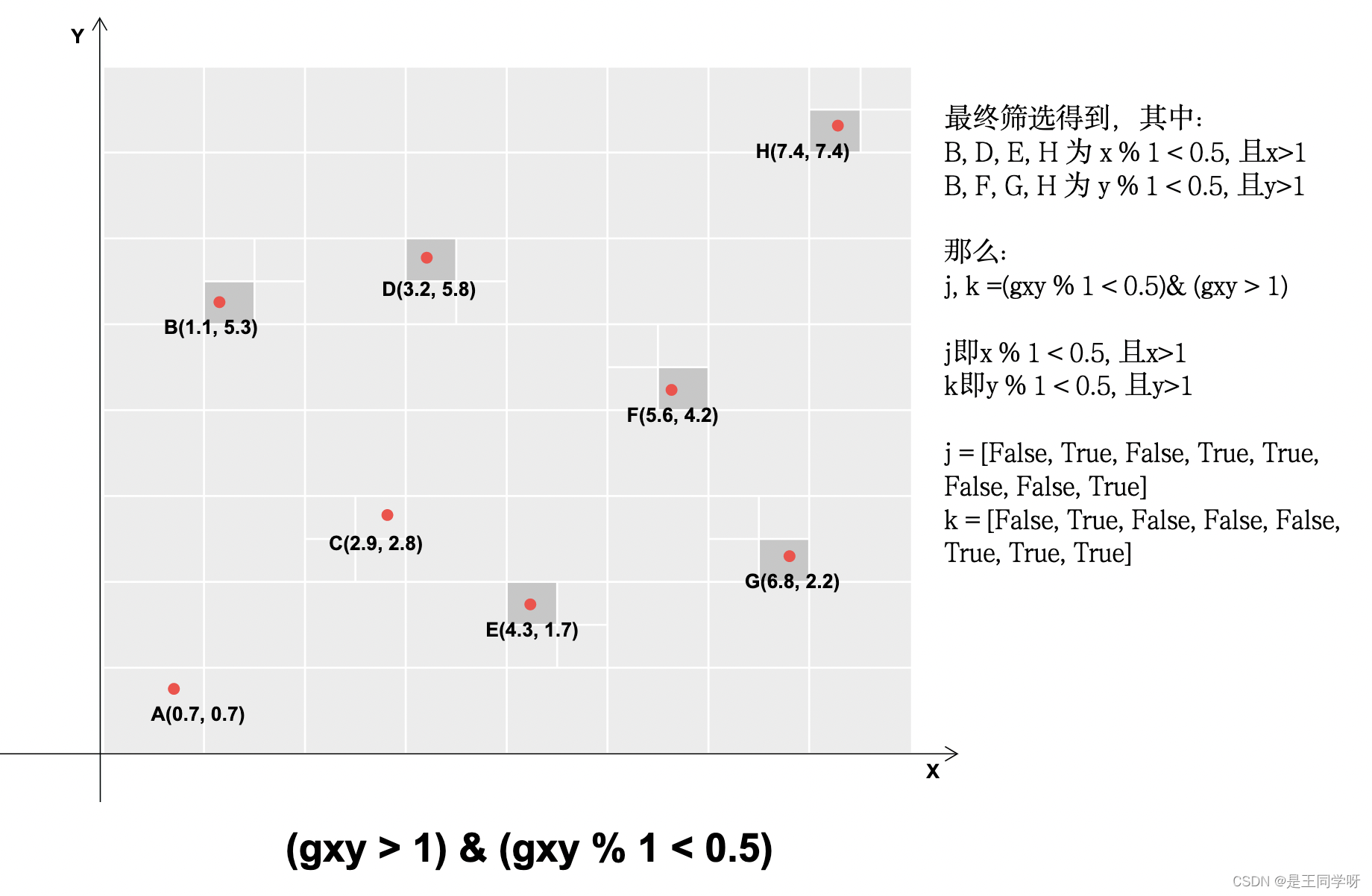
(gxi %1< g)&(gxi >1)# 条件合并得到下图

j = torch.stack((torch.ones_like(j), j, k, l, m))
t = t.repeat((5,1,1))[j]# yolov5不仅用目标中心点所在的网格预测该目标，还采用了距目标中心点的最近两个网格# 所以有五种情况，网格本身，上下左右|----------------------------------------------------------------------||            这里将t复制5个，然后使用j来过滤                                      ||    第一个t是保留经过第一步过滤留下的gtbox，因为上一步里面增加了一个全为true的维度||            第二个t保留了靠近方格左边的gtbox，                               ||            第三个t保留了靠近方格上方的gtbox，                               ||            第四个t保留了靠近方格右边的gtbox，                               ||            第五个t保留了靠近方格下边的gtbox，                               ||----------------------------------------------------------------------|
offsets =(torch.zeros_like(gxy)[None] + off[:, None])[j]# 生成偏移矩阵

j的第一行全为1，意思是指经过第一步保留下的bbox所在的grid_cell为1.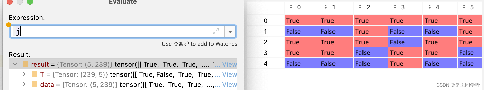

else:
     t = targets[0]
     offsets =0

# Define
 bc, gxy, gwh, a = t.chunk(4,1)# (image, class), grid xy, grid wh, anchors
 a,(b, c)= a.long().view(-1), bc.long().T  # anchors, image, class
 gij =(gxy - offsets).long()#减去偏置，得到更多的正样本所在的网格。
 gi, gj = gij.T  # grid indices

下面的四张图展示了

gij = (gxy - offsets).long()

做了啥。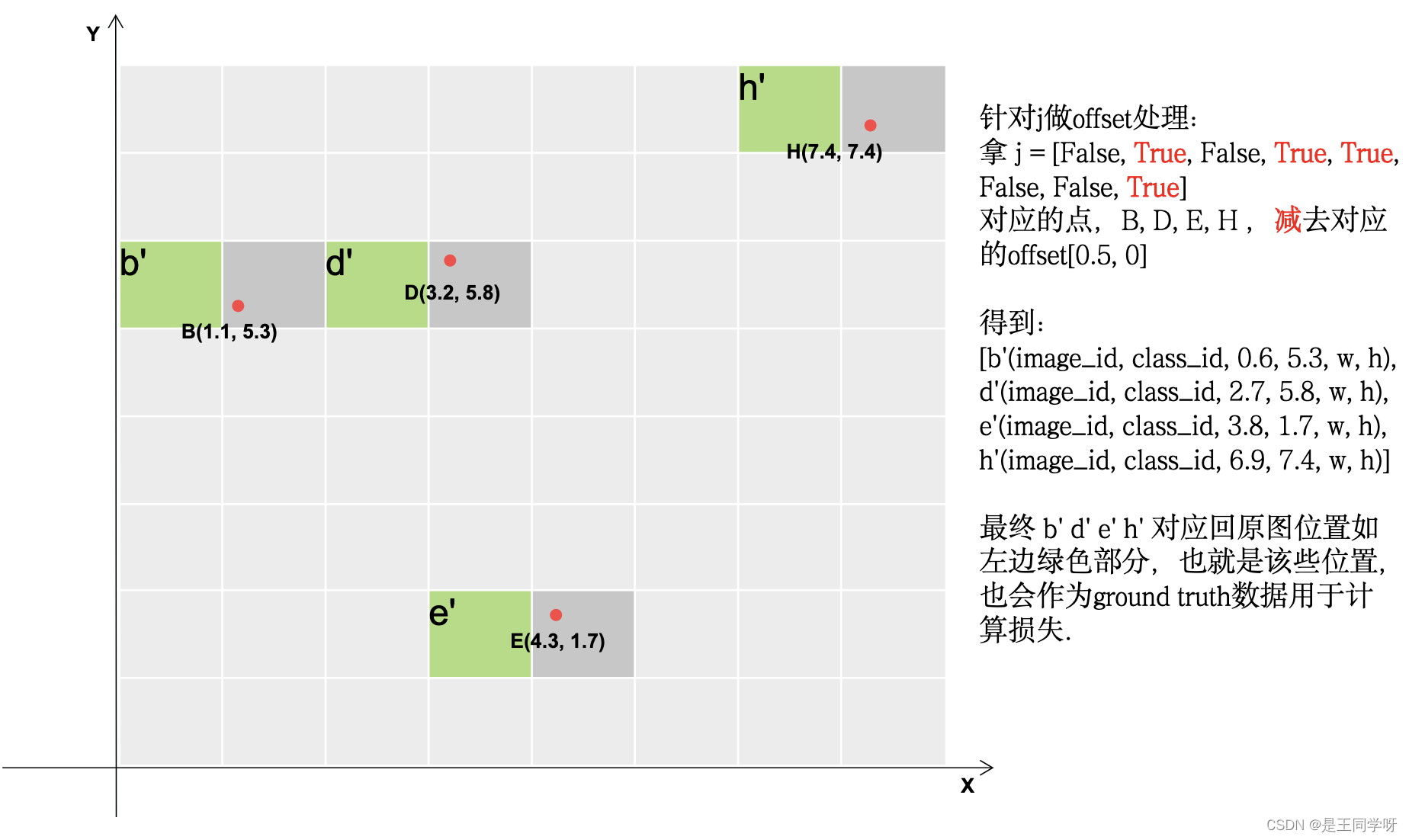




最终得到的结果如下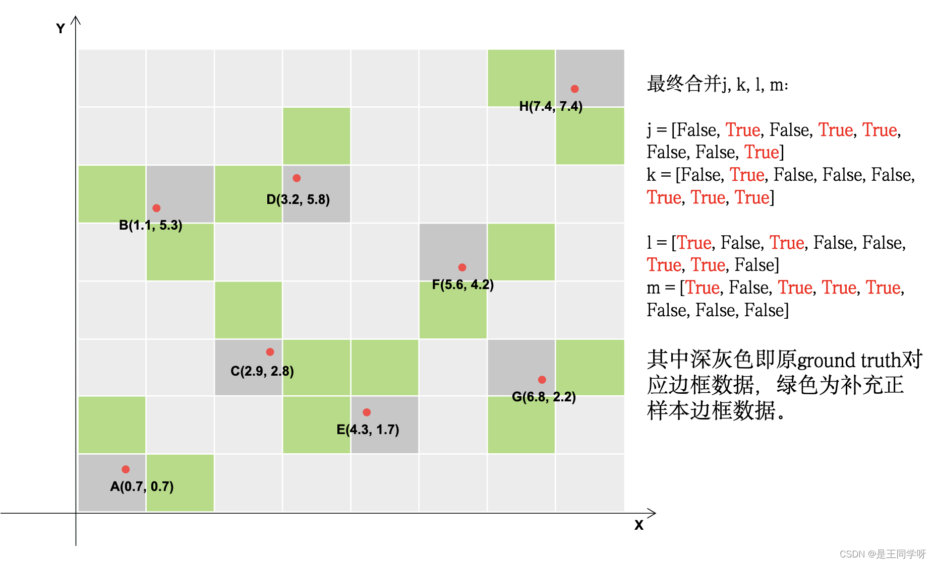

# Append，将对应的结果存储下来。
indices.append((b, a, gj.clamp_(0, gain[3]-1), gi.clamp_(0, gain[2]-1)))# image, anchor, grid indices
tbox.append(torch.cat((gxy - gij, gwh),1))# box
anch.append(anchors[a])# anchors
tcls.append(c)# class

tbox.append(torch.cat((gxy - gij, gwh), 1)) # box

这句话做的如下：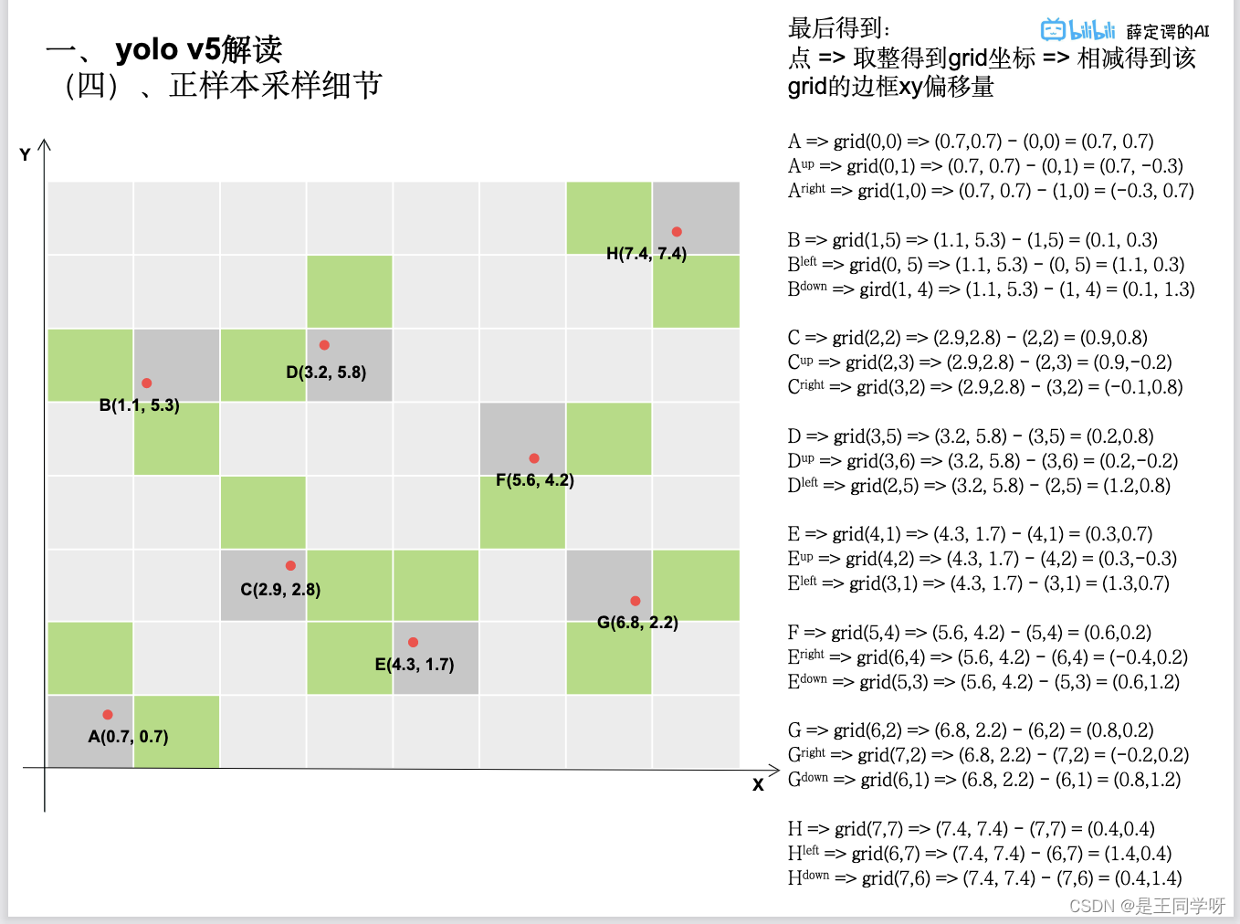

Reference

1. 感谢这位UP主的详细解释，本文的正样本采样细节参考了此UP主的PPT。yolo v5 解读，训练，复现