0


LSTM反向传播原理——LSTM从零实现系列(2)

    LSTM的反向传播过程相对复杂,主要因为其对应的控制门较多,而对于每一个控制门我们都需要求导,所以工作量较大。

    首先我们根据LSTM结构图分析一下每个控制门的求导过程。在讲解反向传播之前,先了解一些要用到的参数意义。

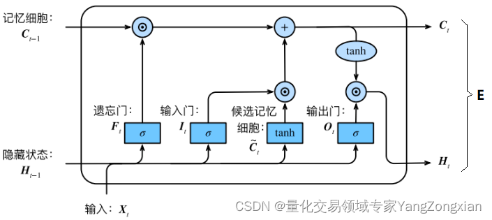
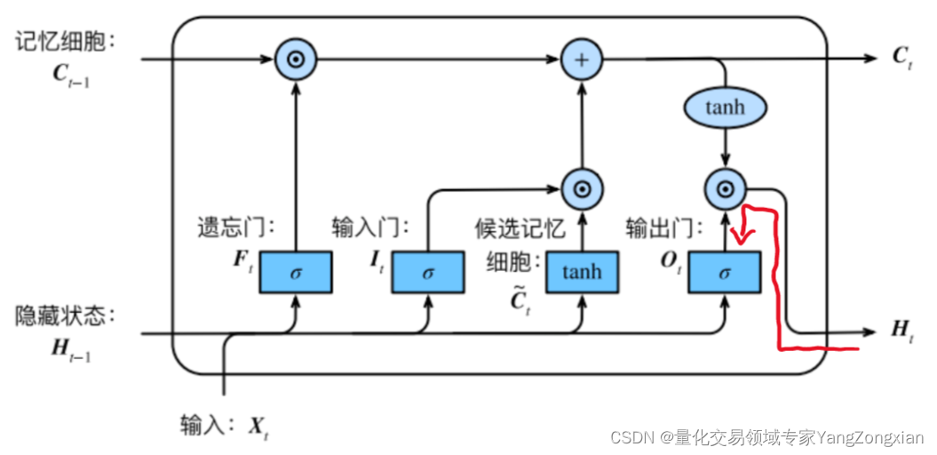
      一般来说LSTM在层后会接一个全连接层FNN,全连接层后面再接一个损失函数Loss,所以这里我将全连接层反向传回给LSTM层的总误差称之为![E](https://latex.codecogs.com/gif.latex?E)。

    从上图LSTM的结构可以观察出,回传的总误差![E](https://latex.codecogs.com/gif.latex?E)其实会由两个分支进入LSTM内部,分别是![C_t](https://latex.codecogs.com/gif.latex?C_t)和![H_t](https://latex.codecogs.com/gif.latex?H_t)。因此从宏观上看,每个LSTM单元误差传播的起始点为![C_t](https://latex.codecogs.com/gif.latex?C_t)和![H_t](https://latex.codecogs.com/gif.latex?H_t),终点为![C_{t-1}](https://latex.codecogs.com/gif.latex?C_%7Bt-1%7D)和![H_{t-1}](https://latex.codecogs.com/gif.latex?H_%7Bt-1%7D),在起始点和终点之间分别夹杂着4个控制门![F ,I ,\tilde{C_t}, O](https://latex.codecogs.com/gif.latex?F%20%2CI%20%2C%5Ctilde%7BC_t%7D%2C%20O),上述的这些元素,其实就是LSTM整个反向传播求导过程要涉及的全部内容。

    下面我们详细介绍每个元素在求导中的处理方法。

二、反向传播过程符号定义和说明

2.1.符号意义说明

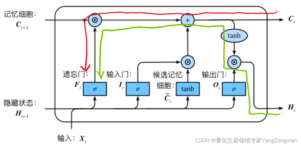
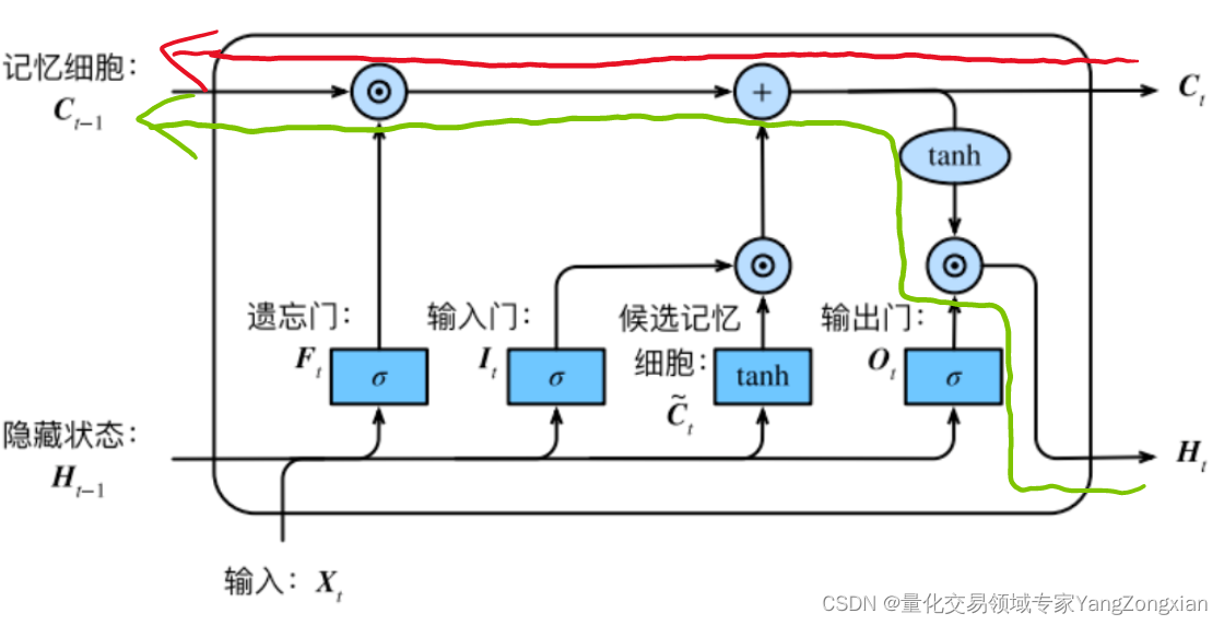
    LSTM单元中误差反向传播的过程大体分为两种情况:一种是反向传播的误差来源只包含![H_t](https://latex.codecogs.com/gif.latex?H_t)一条链,比如控制门![O](https://latex.codecogs.com/gif.latex?O);另一种是反向传播的误差来源包含![C_t](https://latex.codecogs.com/gif.latex?C_t)和![H_t](https://latex.codecogs.com/gif.latex?H_t)两条传播链,比如控制门![F,I,\tilde{C_t}](https://latex.codecogs.com/gif.latex?F%2CI%2C%5Ctilde%7BC_t%7D)以及![C_{t-1}](https://latex.codecogs.com/gif.latex?C_%7Bt-1%7D)。如下图所示的遗忘门![F](https://latex.codecogs.com/gif.latex?F),其反向传播的误差就是来自于红色和绿色两条传播链,计算时两条链都要计算。

    下面我们分别列举各个元素的反向传播路径:

C_{t-1}的误差来自于C_tH_t两条传播链,传播路径为:

\left\{\begin{matrix} E\rightarrow C_t\rightarrow C_{t-1} \\ E\rightarrow H_t\rightarrow C_t\rightarrow C_{t-1} \end{matrix}\right.

H_{t-1}的误差来自于四条传播链,分别对应下面F ,I ,\tilde{C_t}, O四个控制门:

    (1)控制门![O](https://latex.codecogs.com/gif.latex?O)的误差由![H_t](https://latex.codecogs.com/gif.latex?H_t)传来,传播路径为:

E\rightarrow H_t\rightarrow O\rightarrow H_{t-1}

    (2)控制门![F](https://latex.codecogs.com/gif.latex?F)的误差由![H_t](https://latex.codecogs.com/gif.latex?H_t)和![C_t](https://latex.codecogs.com/gif.latex?C_t)传来,传播路径为:

\left\{\begin{matrix} E\rightarrow H_t\rightarrow C_t\rightarrow F\rightarrow H_{t-1} \\ E\rightarrow C_t\rightarrow F\rightarrow H_{t-1} \end{matrix}\right.

   (3)控制门![I](https://latex.codecogs.com/gif.latex?I)的误差由![H_t](https://latex.codecogs.com/gif.latex?H_t)和![C_t](https://latex.codecogs.com/gif.latex?C_t)传来,传播路径为:

\left\{\begin{matrix} E\rightarrow H_t\rightarrow C_t\rightarrow I\rightarrow H_{t-1} \\ E\rightarrow C_t\rightarrow I\rightarrow H_{t-1} \end{matrix}\right.

    (4)控制门![\tilde{C_t}](https://latex.codecogs.com/gif.latex?%5Ctilde%7BC_t%7D)的误差由![H_t](https://latex.codecogs.com/gif.latex?H_t)和![C_t](https://latex.codecogs.com/gif.latex?C_t)传来,传播路径为:

\left\{\begin{matrix} E\rightarrow H_t\rightarrow C_t\rightarrow \tilde{C_t}\rightarrow H_{t-1} \\ E\rightarrow C_t\rightarrow \tilde{C_t}\rightarrow H_{t-1} \end{matrix}\right.

    列举一下每个元素求偏导过程中的符号定义
  1. LSTM单元反向传播的起点C_tH_t的误差,是由上一层传递来的,这里表示为\frac{\partial E}{\partial C_{t}}\frac{\partial E}{\partial H_{t}},是已知常量。
  2. LSTM单元中的H_t是由C_tO_t计算而来,所以求导过程中存在H_tC_t的偏导数 \frac{\partial H_t}{\partial C_{t}},以及 H_tO_t的偏导数 \frac{\partial H_t}{\partial O_{t}}C_t分别由F_t,I_t,\tilde{C_t}计算而来,所以求导过程中存在 C_t分别到F_t,I_t,\tilde{C_t}的偏导数\frac{\partial C_t}{\partial F_{t}}\frac{\partial C_t}{\partial I_{t}}\frac{\partial C_t}{\partial \tilde{C}_{t}}
  3. LSTM单元中从控制门F,I,\tilde{C_t},O_tH_{t-1}存在偏导数\frac{\partial F_t}{\partial H_{t-1}}\frac{\partial I_t}{\partial H_{t-1}}\frac{\partial \tilde{C}_t}{\partial H_{t-1}}\frac{\partial O_t}{\partial H_{t-1}}。从C_tH_tC_{t-1}的偏导数则为\frac{\partial C_t}{\partial C_{t-1}}\frac{\partial H_t}{\partial C_{t-1}}
  4. 最后在求偏导的过程中还会用到一些前向传播的数值,如C_tC_{t-1}F_tI_t等,这些参数在计算前向传播过程中都可以加以保留。
  5. 在理清上述这些反向传播中存在的关系后,下面我们就可以完成整个LSTM单元的反向传播计算了。
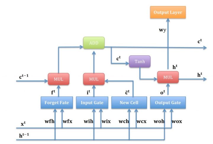
    LSTM计算顺序如下图所示:     

    介绍完这些符号定义后,下面就可以开始LSTM的反向传播计算了。

2.2.重要细节——特殊的传播链Ct

    ![C_t](https://latex.codecogs.com/gif.latex?C_t)是一条比较特殊的传播链,在前向传播时,每个sample都中包含n个Timestep,在第一个Timestep计算时,![C_t](https://latex.codecogs.com/gif.latex?C_t)的初始值是零矩阵,在后续的Timestep计算时![C_t](https://latex.codecogs.com/gif.latex?C_t)会进行不断累计和向后传递。在当前LSTM层计算完成后,向下个LSTM层传递时,只向后传递输出的状态![H_t](https://latex.codecogs.com/gif.latex?H_t),作为下个LSTM层的输入Xh,而当前层的![C_t](https://latex.codecogs.com/gif.latex?C_t)值不再向下个LSTM层传递。

    所以同理,在反向传播时,下一层的![\Delta H_t](https://latex.codecogs.com/gif.latex?%5CDelta%20H_t)会反向传播到上一层作为误差输入,但![\Delta C_t](https://latex.codecogs.com/gif.latex?%5CDelta%20C_t)不会回传,所以每一层LSTM按照时间步倒序计算反向传播过程中,计算第一个Timestep时![\Delta C_t](https://latex.codecogs.com/gif.latex?%5CDelta%20C_t)的初始值也是零矩阵,并且在后续时间步中进行累计和传递。

    这一规则十分重要,在这里单独强调,后续内容不再重复说明。

三、LSTM反向传播流程解析

    上一节我们说过,从反向传播链终点的角度出发,有两种类型的传播链,即 ![C_{t-1}](https://latex.codecogs.com/gif.latex?C_%7Bt-1%7D)链和![H_{t-1}](https://latex.codecogs.com/gif.latex?H_%7Bt-1%7D)链 。而细分![H_{t-1}](https://latex.codecogs.com/gif.latex?H_%7Bt-1%7D)的传播链其实又有两种类型,即包含![C_t](https://latex.codecogs.com/gif.latex?C_t)的和不包含![C_t](https://latex.codecogs.com/gif.latex?C_t)的。所以反向传播链大体上可分为三类,下面来讲解这三种流程。

3.1.第一类偏导:H_{F}H_{I}H_{\tilde{C}}

3.1.1.遗忘门F_t求导过程

    两条完整求导路径表达式如下

\frac{\partial E}{\partial H_{t-1}}=\frac{\partial E}{\partial C_{t}}\cdot \frac{\partial C_{t}}{\partial F_{t}}\cdot \frac{\partial F_t}{\partial H_{t-1}}+\frac{\partial E}{\partial H_{t}}\cdot\frac{\partial H_{t}}{\partial C_{t}}\cdot \frac{\partial C_{t}}{\partial F_{t}}\cdot \frac{\partial F_t}{\partial H_{t-1}}

\frac{\partial E}{\partial H_{t-1}}= (\frac{\partial E}{\partial C_{t}}+\frac{\partial E}{\partial H_{t}}\cdot\frac{\partial H_{t}}{\partial C_{t}})\cdot \frac{\partial C_{t}}{\partial F_{t}}\cdot \frac{\partial F_t}{\partial H_{t-1}}

    **3.1.1.1.**绿色路径![H_t](https://latex.codecogs.com/gif.latex?H_t)到![C_t](https://latex.codecogs.com/gif.latex?C_t)的偏导

H_t=O_t\odot tan(C_t)

\frac{\partial H_t}{\partial C_t}=O_t\odot (1-tan^{2}C_t)

    **3.1.1.2.**红色路径![C_t](https://latex.codecogs.com/gif.latex?C_t)到![F_t](https://latex.codecogs.com/gif.latex?F_t)的偏导 

C_t=F_t\odot C_{t-1}+I_t\odot \tilde{C_t}

\frac{\partial C_t}{\partial F_t}=C_{t-1}

    **3.1.1.3.**遗忘门![F_t](https://latex.codecogs.com/gif.latex?F_t)到![H_{t-1}](https://latex.codecogs.com/gif.latex?H_%7Bt-1%7D)的偏导 

F_{t}=\sigma (x_{t}W_{xf}+h_{t-1}W_{h_{t-1}f}+b_f)

{\sigma}'(x)=\sigma (x)(1-\sigma (x))

\frac{\partial F_t}{\partial H_{t-1}}=F_t(1-F_t)

    **3.1.1.4.**两条路径表达式合并

\frac{\partial E}{\partial H_{t-1}}= \left \{ \frac{\partial E}{\partial C_{t}}+\frac{\partial E}{\partial H_{t}}\cdot[O_t\odot (1-tan^{2}C_t)] \right \}\cdot C_{t-1}\cdot F_t(1-F_t)

3.1.2.输入门I_t求导过程

    原理同上,这里直接写

\frac{\partial E}{\partial H_{t-1}}=\frac{\partial E}{\partial C_{t}}\cdot \frac{\partial C_{t}}{\partial I_{t}}\cdot \frac{\partial I_t}{\partial H_{t-1}}+\frac{\partial E}{\partial H_{t}}\cdot\frac{\partial H_{t}}{\partial C_{t}}\cdot \frac{\partial C_{t}}{\partial I_{t}}\cdot \frac{\partial I_t}{\partial H_{t-1}}

\frac{\partial E}{\partial H_{t-1}}= (\frac{\partial E}{\partial C_{t}}+\frac{\partial E}{\partial H_{t}}\cdot\frac{\partial H_{t}}{\partial C_{t}})\cdot \frac{\partial C_{t}}{\partial I_{t}}\cdot \frac{\partial I_t}{\partial H_{t-1}}

** 3.1.2.1.**H_tC_t的偏导

H_t=O_t\odot tan(C_t)

\frac{\partial H_t}{\partial C_t}=O_t\odot (1-tan^{2}C_t)

    **3.1.2.2.**![C_t](https://latex.codecogs.com/gif.latex?C_t)到![I_t](https://latex.codecogs.com/gif.latex?I_t)的偏导 

C_t=F_t\odot C_{t-1}+I_t\odot \tilde{C_t}

\frac{\partial C_t}{\partial I_t}=\tilde{C}_t

    **3.1.2.3.**输入门![I_t](https://latex.codecogs.com/gif.latex?I_t)到![H_{t-1}](https://latex.codecogs.com/gif.latex?H_%7Bt-1%7D)的偏导 

I_{t}=\sigma (x_{t}W_{xI}+h_{t-1}W_{h_{t-1}I}+b_I)

{\sigma}'(x)=\sigma (x)(1-\sigma (x))

\frac{\partial I_t}{\partial H_{t-1}}=I_t(1-I_t)

    **3.1.2.4.**两条路径表达式合并

\frac{\partial E}{\partial H_{t-1}}= \left \{ \frac{\partial E}{\partial C_{t}}+\frac{\partial E}{\partial H_{t}}\cdot[O_t\odot (1-tan^{2}C_t)] \right \}\cdot \tilde{C}_{t}\cdot I_t(1-I_t)

3.1.3.候选记忆\tilde{C}_t求导过程

    原理同上,这里直接写

\frac{\partial E}{\partial H_{t-1}}=\frac{\partial E}{\partial C_{t}}\cdot \frac{\partial C_{t}}{\partial \tilde{C}_{t}}\cdot \frac{\partial \tilde{C}_t}{\partial H_{t-1}}+\frac{\partial E}{\partial H_{t}}\cdot\frac{\partial H_{t}}{\partial C_{t}}\cdot \frac{\partial C_{t}}{\partial \tilde{C}_{t}}\cdot \frac{\partial \tilde{C}_t}{\partial H_{t-1}}

\frac{\partial E}{\partial H_{t-1}}= (\frac{\partial E}{\partial C_{t}}+\frac{\partial E}{\partial H_{t}}\cdot\frac{\partial H_{t}}{\partial C_{t}})\cdot \frac{\partial C_{t}}{\partial \tilde{C}_{t}}\cdot \frac{\partial \tilde{C}_t}{\partial H_{t-1}}

** 3.1.3.1.**H_tC_t的偏导

H_t=O_t\odot tan(C_t)

\frac{\partial H_t}{\partial C_t}=O_t\odot (1-tan^{2}C_t)

    **3.1.3.2.**![C_t](https://latex.codecogs.com/gif.latex?C_t)到![\tilde{C}_t](https://latex.codecogs.com/gif.latex?%5Ctilde%7BC%7D_t)的偏导 

C_t=F_t\odot C_{t-1}+I_t\odot \tilde{C_t}

\frac{\partial C_t}{\partial \tilde{C}_t}=I_t

    **3.1.3.3.**候选记忆![\tilde{C}_t](https://latex.codecogs.com/gif.latex?%5Ctilde%7BC%7D_t)到![H_{t-1}](https://latex.codecogs.com/gif.latex?H_%7Bt-1%7D)的偏导 

\tilde{C_t}=tanh(x_tW_{x\tilde{C}}+h_{t-1}W_{h_{t-1}\tilde{C}}+b_{\tilde{C}})

{\sigma}'(x)=\sigma (x)(1-\sigma (x))

\frac{\partial \tilde{C}_t}{\partial H_{t-1}}=\tilde{C}_t(1-\tilde{C}_t)

    **3.1.3.4.**两条路径表达式合并

\frac{\partial E}{\partial H_{t-1}}= \left \{ \frac{\partial E}{\partial C_{t}}+\frac{\partial E}{\partial H_{t}}\cdot[O_t\odot (1-tan^{2}C_t)] \right \}\cdot I_{t}\cdot \tilde{C}_{t}(1-\tilde{C}_{t})

3.2.第二类偏导:H_{O}

    完成表达式如下 

\frac{\partial E}{\partial H_{t-1}}=\frac{\partial E}{\partial H_t}\cdot \frac{\partial H_t}{\partial O_t}\cdot \frac{\partial O_t}{\partial H_{t-1}}

** 3.2.1.**红色路径H_tO_t偏导

H_t=O_t\odot tan(C_t)

\frac{\partial H_t}{\partial O_t}=tan(C_t)

    **3.2.2.**![O_t](https://latex.codecogs.com/gif.latex?O_t)到![H_{t-1}](https://latex.codecogs.com/gif.latex?H_%7Bt-1%7D)偏导

O_{t}=\sigma (x_{t}W_{xo}+h_{t-1}W_{h_{t-1}o}+b_o)

{\sigma}'(x)=\sigma (x)(1-\sigma (x))

\frac{\partial O_t}{\partial H_{t-1}}=O_t(1-O_t)

    **3.2.3.**表达式合并

\frac{\partial E}{\partial H_{t-1}}=\frac{\partial E}{\partial H_t}\cdot tan(C_t)\cdot O_t(1-O_t)

3.3.第三类偏导:C_{t-1}

    两条完整求导路径表达式如下

\frac{\partial E}{\partial C_{t-1}}=\frac{\partial E }{\partial C_{t}}\cdot \frac{\partial C_{t}}{\partial C_{t-1}}+\frac{\partial E}{\partial H_{t}}\cdot\frac{\partial H_{t}}{\partial C_{t}}\cdot \frac{\partial C_{t}}{\partial C_{t-1}}

\frac{\partial E}{\partial C_{t-1}}=(\frac{\partial E}{\partial C_{t}}+\frac{\partial E}{\partial H_{t}}\cdot\frac{\partial H_{t}}{\partial C_{t}})\cdot \frac{\partial C_{t}}{\partial C_{t-1}}

** 3.3.1.**红色路径C_tC_{t-1}的偏导

C_t=F_t\odot C_{t-1}+I_t\odot \tilde{C_t}

\frac{\partial C_t}{\partial C_{t-1}}=F_{t}

** 3.3.2.**绿色路径H_tC_t的偏导

H_t=O_t\odot tan(C_t)

\frac{\partial H_t}{\partial C_t}=O_t\left [ 1-tan^{2}(C_t) \right ]

** 3.3.3.**两条路径表达式合并

\frac{\partial E}{\partial C_{t-1}}=\left \{ \frac{\partial E}{\partial C_{t}}+\frac{\partial E}{\partial H_{t}}\cdot O_t\left [ 1-tan^{2}(C_t) \right ] \right \}\cdot F_t

3.4.合并

    四个控制门计算完成后,最终合并起来,表达式如下:

\frac{\partial E}{\partial Sum}=\frac{\partial E}{\partial F}+\frac{\partial E}{\partial I}+\frac{\partial E}{\partial \tilde{C}}+\frac{\partial E}{\partial O}

四、权重的反向传播

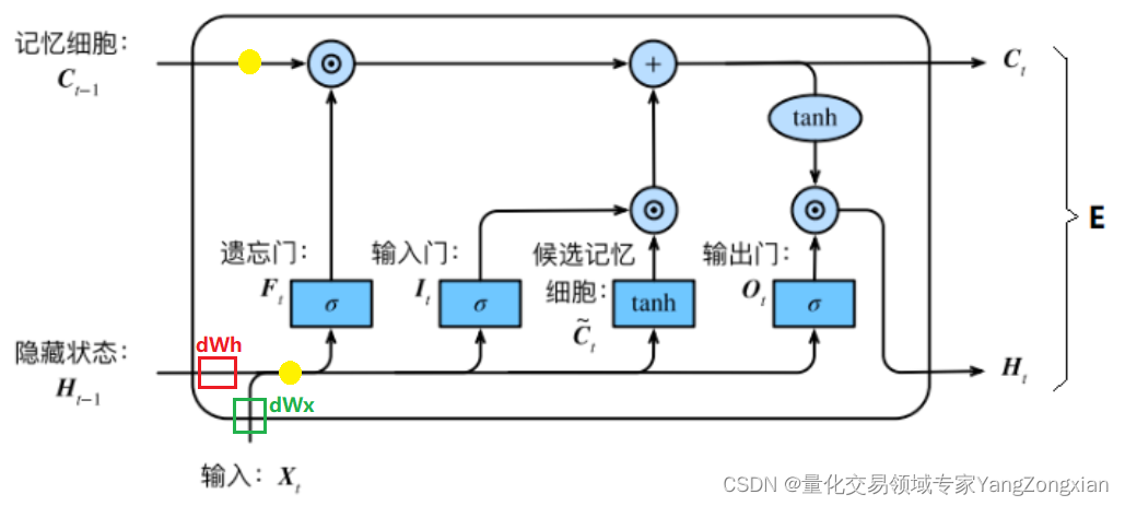
    在上述第三节的求导过程结束后,此时误差就传递到了上图中的两个黄色圆圈部分,显然还差一步反向传播就完成了。最后一步就是将误差从黄色的圆圈部分分别传递到![C_{t-1}](https://latex.codecogs.com/gif.latex?C_%7Bt-1%7D),![H_{t-1}](https://latex.codecogs.com/gif.latex?H_%7Bt-1%7D),![X_t](https://latex.codecogs.com/gif.latex?X_t)。对于![H_{t-1}](https://latex.codecogs.com/gif.latex?H_%7Bt-1%7D)和![X_t](https://latex.codecogs.com/gif.latex?X_t)来说,要计算两个权重矩阵![\Delta W_h](https://latex.codecogs.com/gif.latex?%5CDelta%20W_h)和![\Delta W_x](https://latex.codecogs.com/gif.latex?%5CDelta%20W_x),而对于![C_{t-1}](https://latex.codecogs.com/gif.latex?C_%7Bt-1%7D)来说,不必求矩阵,直接向后传递即可。

    在前向传播时计算流程如下:

\left\{\begin{matrix} H_{t-1}*W_h = Sum_h\\ X_t*W_x = Sum_x \\ Sum_h+Sum_x = Sum \end{matrix}\right.

    由上式可得,反向传播的表达式可以表达如下:

\left\{\begin{matrix} \Delta W_h = (H_{t-1})^T*Sum \\ \Delta H_{t-1}= Sum*(W_h)^T \\ \Delta W_x = (X_t)^T*Sum \\ \Delta X_t = Sum *(W_{x})^T \end{matrix}\right.

    最后还剩一个偏置项![b](https://latex.codecogs.com/gif.latex?b),我们将上一节得出的![\frac{\partial E}{\partial Sum}](https://latex.codecogs.com/gif.latex?%5Cfrac%7B%5Cpartial%20E%7D%7B%5Cpartial%20Sum%7D)直接降维即可得到![\Delta b](https://latex.codecogs.com/gif.latex?%5CDelta%20b),具体的程序实现方法会在下一篇文章中更直观的介绍。

五、总结

    上面就是一个完整的LSTM单元反向传播流程,至此本文已经对LSTM的反向传播理论基础进行了比较清楚的讲解。结合上一篇LSTM网络前向传播原理讲解,相信大家对LSTM的基本原理有了一个比较清晰的认识了。

    但这仅仅是单一的LSTM模型前向传播和反向传播原理,不足以构成一个完整的模型。但是有了上述基础,下篇文章中我们就可以1:1实现一个包含输入,隐藏层,输出,损失函数的完整的神经网络模型了。

文章正在写作中……

参考文献:

循环神经网络RNN&LSTM推导及实现 - 知乎

LSTM的推导与实现 - liujshi - 博客园

RNN、LSTM反向传播推导详解 - 灰信网(软件开发博客聚合)

手推公式:LSTM单元梯度的详细的数学推导

LSTM –随时间反向传播的推导 - 芒果文档


本文转载自: https://blog.csdn.net/yangwohenmai1/article/details/128047225
版权归原作者 日拱一两卒 所有, 如有侵权,请联系我们删除。

“LSTM反向传播原理——LSTM从零实现系列(2)”的评论:

还没有评论