
睿智的目标检测60——Pytorch搭建YoloV7目标检测平台
学习前言
AB哥弄了个YoloV7,我觉得有必要跟进看看,它的concat结构还是第一次见,感觉有点意思。
源码下载
https://github.com/bubbliiiing/yolov7-pytorch
喜欢的可以点个star噢。
YoloV7改进的部分(不完全)
1、主干部分:使用了创新的多分支堆叠结构进行特征提取,相比以前的Yolo,模型的跳连接结构更加的密集。使用了创新的下采样结构,使用Maxpooling和步长为2x2的特征并行进行提取与压缩。
2、加强特征提取部分:同主干部分,加强特征提取部分也使用了多输入堆叠结构进行特征提取,使用Maxpooling和步长为2x2的特征并行进行下采样。
3、特殊的SPP结构:使用了具有CSP机构的SPP扩大感受野,在SPP结构中引入了CSP结构,该模块具有一个大的残差边辅助优化与特征提取。
4、自适应多正样本匹配:在YoloV5之前的Yolo系列里面,在训练时每一个真实框对应一个正样本,即在训练时,每一个真实框仅由一个先验框负责预测。YoloV7中为了加快模型的训练效率,增加了正样本的数量,在训练时,每一个真实框可以由多个先验框负责预测。除此之外,对于每个真实框,还会根据先验框调整后的预测框进行iou与种类的计算,获得cost,进而找到最适合该真实框的先验框。
5、借鉴了RepVGG的结构,在网络的特定部分引入RepConv,fuse后在保证网络x减少网络的参数量
6、使用了辅助分支辅助收敛,但是在模型较小的YoloV7和YoloV7-X中并没有使用。
以上并非全部的改进部分,还存在一些其它的改进,这里只列出来了一些我比较感兴趣,而且非常有效的改进。
YoloV7实现思路
一、整体结构解析

在学习YoloV7之前,我们需要对YoloV7所作的工作有一定的了解,这有助于我们后面去了解网络的细节,YoloV7在预测方式上与之前的Yolo并没有多大的差别,依然分为三个部分。
分别是Backbone,FPN以及Yolo Head。
Backbone是YoloV7的主干特征提取网络,输入的图片首先会在主干网络里面进行特征提取,提取到的特征可以被称作特征层,是输入图片的特征集合。在主干部分,我们获取了三个特征层进行下一步网络的构建,这三个特征层我称它为有效特征层。
FPN是YoloV7的加强特征提取网络,在主干部分获得的三个有效特征层会在这一部分进行特征融合,特征融合的目的是结合不同尺度的特征信息。在FPN部分,已经获得的有效特征层被用于继续提取特征。在YoloV7里依然使用到了Panet的结构,我们不仅会对特征进行上采样实现特征融合,还会对特征再次进行下采样实现特征融合。
Yolo Head是YoloV7的分类器与回归器,通过Backbone和FPN,我们已经可以获得三个加强过的有效特征层。每一个特征层都有宽、高和通道数,此时我们可以将特征图看作一个又一个特征点的集合,每个特征点上有三个先验框,每一个先验框都有通道数个特征。Yolo Head实际上所做的工作就是对特征点进行判断,判断特征点上的先验框是否有物体与其对应。与以前版本的Yolo一样,YoloV7所用的解耦头是一起的,也就是分类和回归在一个1X1卷积里实现。
因此,整个YoloV7网络所作的工作就是 特征提取-特征加强-预测先验框对应的物体情况。
二、网络结构解析
1、主干网络Backbone介绍
YoloV7所使用的主干特征提取网络具有两个重要特点:
1、使用了多分支堆叠模块,这个模块其实论文里没有命名,但是我在分析源码后认为这个名字非常合适,在本博文中,多分支堆叠模块如图所示。
看了这幅图大家应该明白为什么我把这个模块称为多分支堆叠模块,因为在该模块中,最终堆叠模块的输入包含多个分支,左一为一个卷积标准化激活函数,左二为一个卷积标准化激活函数,右二为三个卷积标准化激活函数,右一为五个卷积标准化激活函数。
四个特征层在堆叠后会再次进行一个卷积标准化激活函数来特征整合。
classMulti_Concat_Block(nn.Module):def__init__(self, c1, c2, c3, n=4, e=1, ids=[0]):super(Multi_Concat_Block, self).__init__()
        c_ =int(c2 * e)

        self.ids = ids
        self.cv1 = Conv(c1, c_,1,1)
        self.cv2 = Conv(c1, c_,1,1)
        self.cv3 = nn.ModuleList([Conv(c_ if i ==0else c2, c2,3,1)for i inrange(n)])
        self.cv4 = Conv(c_ *2+ c2 *(len(ids)-2), c3,1,1)defforward(self, x):
        x_1 = self.cv1(x)
        x_2 = self.cv2(x)

        x_all =[x_1, x_2]for i inrange(len(self.cv3)):
            x_2 = self.cv3[i](x_2)
            x_all.append(x_2)

        out = self.cv4(torch.cat([x_all[id]foridin self.ids],1))return out
如此多的堆叠其实也对应了更密集的残差结构,残差网络的特点是容易优化,并且能够通过增加相当的深度来提高准确率。其内部的残差块使用了跳跃连接,缓解了在深度神经网络中增加深度带来的梯度消失问题。
2、使用创新的过渡模块Transition_Block来进行下采样,在卷积神经网络中,常见的用于下采样的过渡模块是一个卷积核大小为3x3、步长为2x2的卷积或者一个步长为2x2的最大池化。在YoloV7中,作者将两种过渡模块进行了集合,一个过渡模块存在两个分支,如图所示。左分支是一个步长为2x2的最大池化+一个1x1卷积,右分支是一个1x1卷积+一个卷积核大小为3x3、步长为2x2的卷积,两个分支的结果在输出时会进行堆叠。
classMP(nn.Module):def__init__(self, k=2):super(MP, self).__init__()
        self.m = nn.MaxPool2d(kernel_size=k, stride=k)defforward(self, x):return self.m(x)classTransition_Block(nn.Module):def__init__(self, c1, c2):super(Transition_Block, self).__init__()
        self.cv1 = Conv(c1, c2,1,1)
        self.cv2 = Conv(c1, c2,1,1)
        self.cv3 = Conv(c2, c2,3,2)

        self.mp  = MP()defforward(self, x):
        x_1 = self.mp(x)
        x_1 = self.cv1(x_1)

        x_2 = self.cv2(x)
        x_2 = self.cv3(x_2)return torch.cat([x_2, x_1],1)
整个主干实现代码为:
import torch
import torch.nn as nn

defautopad(k, p=None):if p isNone:
        p = k //2ifisinstance(k,int)else[x //2for x in k]return p

classSiLU(nn.Module):@staticmethoddefforward(x):return x * torch.sigmoid(x)classConv(nn.Module):def__init__(self, c1, c2, k=1, s=1, p=None, g=1, act=SiLU()):# ch_in, ch_out, kernel, stride, padding, groupssuper(Conv, self).__init__()
        self.conv   = nn.Conv2d(c1, c2, k, s, autopad(k, p), groups=g, bias=False)
        self.bn     = nn.BatchNorm2d(c2, eps=0.001, momentum=0.03)
        self.act    = nn.LeakyReLU(0.1, inplace=True)if act isTrueelse(act ifisinstance(act, nn.Module)else nn.Identity())defforward(self, x):return self.act(self.bn(self.conv(x)))deffuseforward(self, x):return self.act(self.conv(x))classMulti_Concat_Block(nn.Module):def__init__(self, c1, c2, c3, n=4, e=1, ids=[0]):super(Multi_Concat_Block, self).__init__()
        c_ =int(c2 * e)

        self.ids = ids
        self.cv1 = Conv(c1, c_,1,1)
        self.cv2 = Conv(c1, c_,1,1)
        self.cv3 = nn.ModuleList([Conv(c_ if i ==0else c2, c2,3,1)for i inrange(n)])
        self.cv4 = Conv(c_ *2+ c2 *(len(ids)-2), c3,1,1)defforward(self, x):
        x_1 = self.cv1(x)
        x_2 = self.cv2(x)

        x_all =[x_1, x_2]for i inrange(len(self.cv3)):
            x_2 = self.cv3[i](x_2)
            x_all.append(x_2)

        out = self.cv4(torch.cat([x_all[id]foridin self.ids],1))return out

classMP(nn.Module):def__init__(self, k=2):super(MP, self).__init__()
        self.m = nn.MaxPool2d(kernel_size=k, stride=k)defforward(self, x):return self.m(x)classTransition_Block(nn.Module):def__init__(self, c1, c2):super(Transition_Block, self).__init__()
        self.cv1 = Conv(c1, c2,1,1)
        self.cv2 = Conv(c1, c2,1,1)
        self.cv3 = Conv(c2, c2,3,2)

        self.mp  = MP()defforward(self, x):
        x_1 = self.mp(x)
        x_1 = self.cv1(x_1)

        x_2 = self.cv2(x)
        x_2 = self.cv3(x_2)return torch.cat([x_2, x_1],1)classBackbone(nn.Module):def__init__(self, transition_channels, block_channels, n, phi, pretrained=False):super().__init__()#-----------------------------------------------##   输入图片是640, 640, 3#-----------------------------------------------#
        ids ={'l':[-1,-3,-5,-6],'x':[-1,-3,-5,-7,-8],}[phi]
        self.stem = nn.Sequential(
            Conv(3, transition_channels,3,1),
            Conv(transition_channels, transition_channels *2,3,2),
            Conv(transition_channels *2, transition_channels *2,3,1),)
        self.dark2 = nn.Sequential(
            Conv(transition_channels *2, transition_channels *4,3,2),
            Multi_Concat_Block(transition_channels *4, block_channels *2, transition_channels *8, n=n, ids=ids),)
        self.dark3 = nn.Sequential(
            Transition_Block(transition_channels *8, transition_channels *4),
            Multi_Concat_Block(transition_channels *8, block_channels *4, transition_channels *16, n=n, ids=ids),)
        self.dark4 = nn.Sequential(
            Transition_Block(transition_channels *16, transition_channels *8),
            Multi_Concat_Block(transition_channels *16, block_channels *8, transition_channels *32, n=n, ids=ids),)
        self.dark5 = nn.Sequential(
            Transition_Block(transition_channels *32, transition_channels *16),
            Multi_Concat_Block(transition_channels *32, block_channels *8, transition_channels *32, n=n, ids=ids),)if pretrained:
            url ={"l":'https://github.com/bubbliiiing/yolov7-pytorch/releases/download/v1.0/yolov7_backbone_weights.pth',"x":'https://github.com/bubbliiiing/yolov7-pytorch/releases/download/v1.0/yolov7_x_backbone_weights.pth',}[phi]
            checkpoint = torch.hub.load_state_dict_from_url(url=url, map_location="cpu", model_dir="./model_data")
            self.load_state_dict(checkpoint, strict=False)print("Load weights from "+ url.split('/')[-1])defforward(self, x):
        x = self.stem(x)
        x = self.dark2(x)#-----------------------------------------------##   dark3的输出为80, 80, 256,是一个有效特征层#-----------------------------------------------#
        x = self.dark3(x)
        feat1 = x
        #-----------------------------------------------##   dark4的输出为40, 40, 512,是一个有效特征层#-----------------------------------------------#
        x = self.dark4(x)
        feat2 = x
        #-----------------------------------------------##   dark5的输出为20, 20, 1024,是一个有效特征层#-----------------------------------------------#
        x = self.dark5(x)
        feat3 = x
        return feat1, feat2, feat3
2、构建FPN特征金字塔进行加强特征提取
在特征利用部分,YoloV7提取多特征层进行目标检测,一共提取三个特征层。
三个特征层位于主干部分的不同位置,分别位于中间层,中下层,底层,当输入为(640,640,3)的时候,三个特征层的shape分别为feat1=(80,80,256)、feat2=(40,40,512)、feat3=(20,20,1024)。
在获得三个有效特征层后,我们利用这三个有效特征层进行FPN层的构建,构建方式为(在本博文中,将SPPCSPC结构归于FPN中):
- feat3=(20,20,1024)的特征层首先利用SPPCSPC进行特征提取,该结构可以提高YoloV7的感受野,获得P5。
- 对P5先进行1次1X1卷积调整通道,然后进行上采样UmSampling2d后与feat2=(40,40,512)进行一次卷积后的特征层进行结合,然后使用Multi_Concat_Block进行特征提取获得P4,此时获得的特征层为(40,40,512)。
- 对P4先进行1次1X1卷积调整通道,然后进行上采样UmSampling2d后与feat1=(80,80,256)进行一次卷积后的特征层进行结合,然后使用Multi_Concat_Block进行特征提取获得P3_out,此时获得的特征层为(80,80,256)。
- P3_out=(80,80,256)的特征层进行一次Transition_Block卷积进行下采样,下采样后与P4堆叠,然后使用Multi_Concat_Block进行特征提取P4_out,此时获得的特征层为(40,40,512)。
- P4_out=(40,40,512)的特征层进行一次Transition_Block卷积进行下采样,下采样后与P5堆叠,然后使用Multi_Concat_Block进行特征提取P5_out,此时获得的特征层为(20,20,1024)。
特征金字塔可以将不同shape的特征层进行特征融合,有利于提取出更好的特征。
#---------------------------------------------------##   yolo_body#---------------------------------------------------#classYoloBody(nn.Module):def__init__(self, anchors_mask, num_classes, phi, pretrained=False):super(YoloBody, self).__init__()#-----------------------------------------------##   定义了不同yolov7版本的参数#-----------------------------------------------#
        transition_channels ={'l':32,'x':40}[phi]
        block_channels      =32
        panet_channels      ={'l':32,'x':64}[phi]
        e       ={'l':2,'x':1}[phi]
        n       ={'l':4,'x':6}[phi]
        ids     ={'l':[-1,-2,-3,-4,-5,-6],'x':[-1,-3,-5,-7,-8]}[phi]
        conv    ={'l': RepConv,'x': Conv}[phi]#-----------------------------------------------##   输入图片是640, 640, 3#-----------------------------------------------##---------------------------------------------------#   #   生成主干模型#   获得三个有效特征层,他们的shape分别是:#   80, 80, 512#   40, 40, 1024#   20, 20, 1024#---------------------------------------------------#
        self.backbone   = Backbone(transition_channels, block_channels, n, phi, pretrained=pretrained)

        self.upsample   = nn.Upsample(scale_factor=2, mode="nearest")

        self.sppcspc                = SPPCSPC(transition_channels *32, transition_channels *16)
        self.conv_for_P5            = Conv(transition_channels *16, transition_channels *8)
        self.conv_for_feat2         = Conv(transition_channels *32, transition_channels *8)
        self.conv3_for_upsample1    = Multi_Concat_Block(transition_channels *16, panet_channels *4, transition_channels *8, e=e, n=n, ids=ids)

        self.conv_for_P4            = Conv(transition_channels *8, transition_channels *4)
        self.conv_for_feat1         = Conv(transition_channels *16, transition_channels *4)
        self.conv3_for_upsample2    = Multi_Concat_Block(transition_channels *8, panet_channels *2, transition_channels *4, e=e, n=n, ids=ids)

        self.down_sample1           = Transition_Block(transition_channels *4, transition_channels *4)
        self.conv3_for_downsample1  = Multi_Concat_Block(transition_channels *16, panet_channels *4, transition_channels *8, e=e, n=n, ids=ids)

        self.down_sample2           = Transition_Block(transition_channels *8, transition_channels *8)
        self.conv3_for_downsample2  = Multi_Concat_Block(transition_channels *32, panet_channels *8, transition_channels *16, e=e, n=n, ids=ids)

        self.rep_conv_1 = conv(transition_channels *4, transition_channels *8,3,1)
        self.rep_conv_2 = conv(transition_channels *8, transition_channels *16,3,1)
        self.rep_conv_3 = conv(transition_channels *16, transition_channels *32,3,1)

        self.yolo_head_P3 = nn.Conv2d(transition_channels *8,len(anchors_mask[2])*(5+ num_classes),1)
        self.yolo_head_P4 = nn.Conv2d(transition_channels *16,len(anchors_mask[1])*(5+ num_classes),1)
        self.yolo_head_P5 = nn.Conv2d(transition_channels *32,len(anchors_mask[0])*(5+ num_classes),1)deffuse(self):print('Fusing layers... ')for m in self.modules():ifisinstance(m, RepConv):
                m.fuse_repvgg_block()eliftype(m)is Conv andhasattr(m,'bn'):
                m.conv = fuse_conv_and_bn(m.conv, m.bn)delattr(m,'bn')
                m.forward = m.fuseforward
        return self

    defforward(self, x):#  backbone
        feat1, feat2, feat3 = self.backbone.forward(x)

        P5          = self.sppcspc(feat3)
        P5_conv     = self.conv_for_P5(P5)
        P5_upsample = self.upsample(P5_conv)
        P4          = torch.cat([self.conv_for_feat2(feat2), P5_upsample],1)
        P4          = self.conv3_for_upsample1(P4)

        P4_conv     = self.conv_for_P4(P4)
        P4_upsample = self.upsample(P4_conv)
        P3          = torch.cat([self.conv_for_feat1(feat1), P4_upsample],1)
        P3          = self.conv3_for_upsample2(P3)

        P3_downsample = self.down_sample1(P3)
        P4 = torch.cat([P3_downsample, P4],1)
        P4 = self.conv3_for_downsample1(P4)

        P4_downsample = self.down_sample2(P4)
        P5 = torch.cat([P4_downsample, P5],1)
        P5 = self.conv3_for_downsample2(P5)

        P3 = self.rep_conv_1(P3)
        P4 = self.rep_conv_2(P4)
        P5 = self.rep_conv_3(P5)#---------------------------------------------------##   第三个特征层#   y3=(batch_size, 75, 80, 80)#---------------------------------------------------#
        out2 = self.yolo_head_P3(P3)#---------------------------------------------------##   第二个特征层#   y2=(batch_size, 75, 40, 40)#---------------------------------------------------#
        out1 = self.yolo_head_P4(P4)#---------------------------------------------------##   第一个特征层#   y1=(batch_size, 75, 20, 20)#---------------------------------------------------#
        out0 = self.yolo_head_P5(P5)return[out0, out1, out2]
3、利用Yolo Head获得预测结果
利用FPN特征金字塔,我们可以获得三个加强特征,这三个加强特征的shape分别为(20,20,1024)、(40,40,512)、(80,80,256),然后我们利用这三个shape的特征层传入Yolo Head获得预测结果。
与之前Yolo系列不同的是,YoloV7在Yolo Head前使用了一个RepConv的结构,这个RepConv的思想取自于RepVGG,基本思想就是在训练的时候引入特殊的残差结构辅助训练,这个残差结构是经过独特设计的,在实际预测的时候,可以将复杂的残差结构等效于一个普通的3x3卷积,这个时候网络的复杂度就下降了,但网络的预测性能却没有下降。
而对于每一个特征层,我们可以获得利用一个卷积调整通道数,最终的通道数和需要区分的种类个数相关,在YoloV5里,每一个特征层上每一个特征点存在3个先验框。
如果使用的是voc训练集,类则为20种,最后的维度应该为75 = 3x25,三个特征层的shape为(20,20,75),(40,40,75),(80,80,75)。
最后的75可以拆分成3个25,对应3个先验框的25个参数,25可以拆分成4+1+20。
前4个参数用于判断每一个特征点的回归参数,回归参数调整后可以获得预测框;
第5个参数用于判断每一个特征点是否包含物体;
最后20个参数用于判断每一个特征点所包含的物体种类。
如果使用的是coco训练集,类则为80种,最后的维度应该为255 = 3x85,三个特征层的shape为(20,20,255),(40,40,255),(80,80,255)
最后的255可以拆分成3个85,对应3个先验框的85个参数,85可以拆分成4+1+80。
前4个参数用于判断每一个特征点的回归参数,回归参数调整后可以获得预测框;
第5个参数用于判断每一个特征点是否包含物体;
最后80个参数用于判断每一个特征点所包含的物体种类。
实现代码如下:
import numpy as np
import torch
import torch.nn as nn

from nets.backbone import Backbone, Multi_Concat_Block, Conv, SiLU, Transition_Block, autopad

classRepConv(nn.Module):# Represented convolution# https://arxiv.org/abs/2101.03697def__init__(self, c1, c2, k=3, s=1, p=None, g=1, act=SiLU(), deploy=False):super(RepConv, self).__init__()
        self.deploy         = deploy
        self.groups         = g
        self.in_channels    = c1
        self.out_channels   = c2

        assert k ==3assert autopad(k, p)==1

        padding_11  = autopad(k, p)- k //2
        self.act    = nn.LeakyReLU(0.1, inplace=True)if act isTrueelse(act ifisinstance(act, nn.Module)else nn.Identity())if deploy:
            self.rbr_reparam    = nn.Conv2d(c1, c2, k, s, autopad(k, p), groups=g, bias=True)else:
            self.rbr_identity   =(nn.BatchNorm2d(num_features=c1, eps=0.001, momentum=0.03)if c2 == c1 and s ==1elseNone)
            self.rbr_dense      = nn.Sequential(
                nn.Conv2d(c1, c2, k, s, autopad(k, p), groups=g, bias=False),
                nn.BatchNorm2d(num_features=c2, eps=0.001, momentum=0.03),)
            self.rbr_1x1        = nn.Sequential(
                nn.Conv2d( c1, c2,1, s, padding_11, groups=g, bias=False),
                nn.BatchNorm2d(num_features=c2, eps=0.001, momentum=0.03),)defforward(self, inputs):ifhasattr(self,"rbr_reparam"):return self.act(self.rbr_reparam(inputs))if self.rbr_identity isNone:
            id_out =0else:
            id_out = self.rbr_identity(inputs)return self.act(self.rbr_dense(inputs)+ self.rbr_1x1(inputs)+ id_out)defget_equivalent_kernel_bias(self):
        kernel3x3, bias3x3  = self._fuse_bn_tensor(self.rbr_dense)
        kernel1x1, bias1x1  = self._fuse_bn_tensor(self.rbr_1x1)
        kernelid, biasid    = self._fuse_bn_tensor(self.rbr_identity)return(
            kernel3x3 + self._pad_1x1_to_3x3_tensor(kernel1x1)+ kernelid,
            bias3x3 + bias1x1 + biasid,)def_pad_1x1_to_3x3_tensor(self, kernel1x1):if kernel1x1 isNone:return0else:return nn.functional.pad(kernel1x1,[1,1,1,1])def_fuse_bn_tensor(self, branch):if branch isNone:return0,0ifisinstance(branch, nn.Sequential):
            kernel      = branch[0].weight
            running_mean = branch[1].running_mean
            running_var = branch[1].running_var
            gamma       = branch[1].weight
            beta        = branch[1].bias
            eps         = branch[1].eps
        else:assertisinstance(branch, nn.BatchNorm2d)ifnothasattr(self,"id_tensor"):
                input_dim = self.in_channels // self.groups
                kernel_value = np.zeros((self.in_channels, input_dim,3,3), dtype=np.float32
                )for i inrange(self.in_channels):
                    kernel_value[i, i % input_dim,1,1]=1
                self.id_tensor = torch.from_numpy(kernel_value).to(branch.weight.device)
            kernel      = self.id_tensor
            running_mean = branch.running_mean
            running_var = branch.running_var
            gamma       = branch.weight
            beta        = branch.bias
            eps         = branch.eps
        std =(running_var + eps).sqrt()
        t   =(gamma / std).reshape(-1,1,1,1)return kernel * t, beta - running_mean * gamma / std

    defrepvgg_convert(self):
        kernel, bias = self.get_equivalent_kernel_bias()return(
            kernel.detach().cpu().numpy(),
            bias.detach().cpu().numpy(),)deffuse_conv_bn(self, conv, bn):
        std     =(bn.running_var + bn.eps).sqrt()
        bias    = bn.bias - bn.running_mean * bn.weight / std

        t       =(bn.weight / std).reshape(-1,1,1,1)
        weights = conv.weight * t

        bn      = nn.Identity()
        conv    = nn.Conv2d(in_channels = conv.in_channels,
                              out_channels = conv.out_channels,
                              kernel_size = conv.kernel_size,
                              stride=conv.stride,
                              padding = conv.padding,
                              dilation = conv.dilation,
                              groups = conv.groups,
                              bias =True,
                              padding_mode = conv.padding_mode)

        conv.weight = torch.nn.Parameter(weights)
        conv.bias   = torch.nn.Parameter(bias)return conv

    deffuse_repvgg_block(self):if self.deploy:returnprint(f"RepConv.fuse_repvgg_block")
        self.rbr_dense  = self.fuse_conv_bn(self.rbr_dense[0], self.rbr_dense[1])

        self.rbr_1x1    = self.fuse_conv_bn(self.rbr_1x1[0], self.rbr_1x1[1])
        rbr_1x1_bias    = self.rbr_1x1.bias
        weight_1x1_expanded = torch.nn.functional.pad(self.rbr_1x1.weight,[1,1,1,1])# Fuse self.rbr_identityif(isinstance(self.rbr_identity, nn.BatchNorm2d)orisinstance(self.rbr_identity, nn.modules.batchnorm.SyncBatchNorm)):
            identity_conv_1x1 = nn.Conv2d(
                    in_channels=self.in_channels,
                    out_channels=self.out_channels,
                    kernel_size=1,
                    stride=1,
                    padding=0,
                    groups=self.groups,
                    bias=False)
            identity_conv_1x1.weight.data = identity_conv_1x1.weight.data.to(self.rbr_1x1.weight.data.device)
            identity_conv_1x1.weight.data = identity_conv_1x1.weight.data.squeeze().squeeze()
            identity_conv_1x1.weight.data.fill_(0.0)
            identity_conv_1x1.weight.data.fill_diagonal_(1.0)
            identity_conv_1x1.weight.data = identity_conv_1x1.weight.data.unsqueeze(2).unsqueeze(3)

            identity_conv_1x1           = self.fuse_conv_bn(identity_conv_1x1, self.rbr_identity)
            bias_identity_expanded      = identity_conv_1x1.bias
            weight_identity_expanded    = torch.nn.functional.pad(identity_conv_1x1.weight,[1,1,1,1])else:
            bias_identity_expanded      = torch.nn.Parameter( torch.zeros_like(rbr_1x1_bias))
            weight_identity_expanded    = torch.nn.Parameter( torch.zeros_like(weight_1x1_expanded))

        self.rbr_dense.weight   = torch.nn.Parameter(self.rbr_dense.weight + weight_1x1_expanded + weight_identity_expanded)
        self.rbr_dense.bias     = torch.nn.Parameter(self.rbr_dense.bias + rbr_1x1_bias + bias_identity_expanded)

        self.rbr_reparam    = self.rbr_dense
        self.deploy         =Trueif self.rbr_identity isnotNone:del self.rbr_identity
            self.rbr_identity =Noneif self.rbr_1x1 isnotNone:del self.rbr_1x1
            self.rbr_1x1 =Noneif self.rbr_dense isnotNone:del self.rbr_dense
            self.rbr_dense =None#---------------------------------------------------##   yolo_body#---------------------------------------------------#classYoloBody(nn.Module):def__init__(self, anchors_mask, num_classes, phi, pretrained=False):super(YoloBody, self).__init__()#-----------------------------------------------##   定义了不同yolov7版本的参数#-----------------------------------------------#
        transition_channels ={'l':32,'x':40}[phi]
        block_channels      =32
        panet_channels      ={'l':32,'x':64}[phi]
        e       ={'l':2,'x':1}[phi]
        n       ={'l':4,'x':6}[phi]
        ids     ={'l':[-1,-2,-3,-4,-5,-6],'x':[-1,-3,-5,-7,-8]}[phi]
        conv    ={'l': RepConv,'x': Conv}[phi]#-----------------------------------------------##   输入图片是640, 640, 3#-----------------------------------------------##---------------------------------------------------#   #   生成主干模型#   获得三个有效特征层,他们的shape分别是:#   80, 80, 512#   40, 40, 1024#   20, 20, 1024#---------------------------------------------------#
        self.backbone   = Backbone(transition_channels, block_channels, n, phi, pretrained=pretrained)

        self.upsample   = nn.Upsample(scale_factor=2, mode="nearest")

        self.sppcspc                = SPPCSPC(transition_channels *32, transition_channels *16)
        self.conv_for_P5            = Conv(transition_channels *16, transition_channels *8)
        self.conv_for_feat2         = Conv(transition_channels *32, transition_channels *8)
        self.conv3_for_upsample1    = Multi_Concat_Block(transition_channels *16, panet_channels *4, transition_channels *8, e=e, n=n, ids=ids)

        self.conv_for_P4            = Conv(transition_channels *8, transition_channels *4)
        self.conv_for_feat1         = Conv(transition_channels *16, transition_channels *4)
        self.conv3_for_upsample2    = Multi_Concat_Block(transition_channels *8, panet_channels *2, transition_channels *4, e=e, n=n, ids=ids)

        self.down_sample1           = Transition_Block(transition_channels *4, transition_channels *4)
        self.conv3_for_downsample1  = Multi_Concat_Block(transition_channels *16, panet_channels *4, transition_channels *8, e=e, n=n, ids=ids)

        self.down_sample2           = Transition_Block(transition_channels *8, transition_channels *8)
        self.conv3_for_downsample2  = Multi_Concat_Block(transition_channels *32, panet_channels *8, transition_channels *16, e=e, n=n, ids=ids)

        self.rep_conv_1 = conv(transition_channels *4, transition_channels *8,3,1)
        self.rep_conv_2 = conv(transition_channels *8, transition_channels *16,3,1)
        self.rep_conv_3 = conv(transition_channels *16, transition_channels *32,3,1)

        self.yolo_head_P3 = nn.Conv2d(transition_channels *8,len(anchors_mask[2])*(5+ num_classes),1)
        self.yolo_head_P4 = nn.Conv2d(transition_channels *16,len(anchors_mask[1])*(5+ num_classes),1)
        self.yolo_head_P5 = nn.Conv2d(transition_channels *32,len(anchors_mask[0])*(5+ num_classes),1)deffuse(self):print('Fusing layers... ')for m in self.modules():ifisinstance(m, RepConv):
                m.fuse_repvgg_block()eliftype(m)is Conv andhasattr(m,'bn'):
                m.conv = fuse_conv_and_bn(m.conv, m.bn)delattr(m,'bn')
                m.forward = m.fuseforward
        return self

    defforward(self, x):#  backbone
        feat1, feat2, feat3 = self.backbone.forward(x)

        P5          = self.sppcspc(feat3)
        P5_conv     = self.conv_for_P5(P5)
        P5_upsample = self.upsample(P5_conv)
        P4          = torch.cat([self.conv_for_feat2(feat2), P5_upsample],1)
        P4          = self.conv3_for_upsample1(P4)

        P4_conv     = self.conv_for_P4(P4)
        P4_upsample = self.upsample(P4_conv)
        P3          = torch.cat([self.conv_for_feat1(feat1), P4_upsample],1)
        P3          = self.conv3_for_upsample2(P3)

        P3_downsample = self.down_sample1(P3)
        P4 = torch.cat([P3_downsample, P4],1)
        P4 = self.conv3_for_downsample1(P4)

        P4_downsample = self.down_sample2(P4)
        P5 = torch.cat([P4_downsample, P5],1)
        P5 = self.conv3_for_downsample2(P5)

        P3 = self.rep_conv_1(P3)
        P4 = self.rep_conv_2(P4)
        P5 = self.rep_conv_3(P5)#---------------------------------------------------##   第三个特征层#   y3=(batch_size, 75, 80, 80)#---------------------------------------------------#
        out2 = self.yolo_head_P3(P3)#---------------------------------------------------##   第二个特征层#   y2=(batch_size, 75, 40, 40)#---------------------------------------------------#
        out1 = self.yolo_head_P4(P4)#---------------------------------------------------##   第一个特征层#   y1=(batch_size, 75, 20, 20)#---------------------------------------------------#
        out0 = self.yolo_head_P5(P5)return[out0, out1, out2]
三、预测结果的解码
1、获得预测框与得分
由第二步我们可以获得三个特征层的预测结果,shape分别为(N,20,20,255),(N,40,40,255),(N,80,80,255)的数据。
但是这个预测结果并不对应着最终的预测框在图片上的位置,还需要解码才可以完成。在YoloV5里,每一个特征层上每一个特征点存在3个先验框。
每个特征层最后的255可以拆分成3个85,对应3个先验框的85个参数,我们先将其reshape一下,其结果为(N,20,20,3,85),(N,40.40,3,85),(N,80,80,3,85)。
其中的85可以拆分成4+1+80。
前4个参数用于判断每一个特征点的回归参数,回归参数调整后可以获得预测框;
第5个参数用于判断每一个特征点是否包含物体;
最后80个参数用于判断每一个特征点所包含的物体种类。
以(N,20,20,3,85)这个特征层为例,该特征层相当于将图像划分成20x20个特征点,如果某个特征点落在物体的对应框内,就用于预测该物体。
如图所示,蓝色的点为20x20的特征点,此时我们对左图黑色点的三个先验框进行解码操作演示:
1、进行中心预测点的计算,利用Regression预测结果前两个序号的内容对特征点的三个先验框中心坐标进行偏移,偏移后是右图红色的三个点;
2、进行预测框宽高的计算,利用Regression预测结果后两个序号的内容求指数后获得预测框的宽高;
3、此时获得的预测框就可以绘制在图片上了。
除去这样的解码操作,还有非极大抑制的操作需要进行,防止同一种类的框的堆积。
defdecode_box(self, inputs):
    outputs =[]for i,inputinenumerate(inputs):#-----------------------------------------------##   输入的input一共有三个,他们的shape分别是#   batch_size, 255, 20, 20#   batch_size, 255, 40, 40#   batch_size, 255, 80, 80#-----------------------------------------------#
        batch_size      =input.size(0)
        input_height    =input.size(2)
        input_width     =input.size(3)#-----------------------------------------------##   输入为416x416时#   stride_h = stride_w = 32、16、8#-----------------------------------------------#
        stride_h = self.input_shape[0]/ input_height
        stride_w = self.input_shape[1]/ input_width
        #-------------------------------------------------##   此时获得的scaled_anchors大小是相对于特征层的#-------------------------------------------------#
        scaled_anchors =[(anchor_width / stride_w, anchor_height / stride_h)for anchor_width, anchor_height in self.anchors[self.anchors_mask[i]]]#-----------------------------------------------##   输入的input一共有三个,他们的shape分别是#   batch_size, 3, 20, 20, 85#   batch_size, 3, 40, 40, 85#   batch_size, 3, 80, 80, 85#-----------------------------------------------#
        prediction =input.view(batch_size,len(self.anchors_mask[i]),
                                self.bbox_attrs, input_height, input_width).permute(0,1,3,4,2).contiguous()#-----------------------------------------------##   先验框的中心位置的调整参数#-----------------------------------------------#
        x = torch.sigmoid(prediction[...,0])
        y = torch.sigmoid(prediction[...,1])#-----------------------------------------------##   先验框的宽高调整参数#-----------------------------------------------#
        w = torch.sigmoid(prediction[...,2])
        h = torch.sigmoid(prediction[...,3])#-----------------------------------------------##   获得置信度,是否有物体#-----------------------------------------------#
        conf        = torch.sigmoid(prediction[...,4])#-----------------------------------------------##   种类置信度#-----------------------------------------------#
        pred_cls    = torch.sigmoid(prediction[...,5:])

        FloatTensor = torch.cuda.FloatTensor if x.is_cuda else torch.FloatTensor
        LongTensor  = torch.cuda.LongTensor if x.is_cuda else torch.LongTensor

        #----------------------------------------------------------##   生成网格,先验框中心,网格左上角 #   batch_size,3,20,20#----------------------------------------------------------#
        grid_x = torch.linspace(0, input_width -1, input_width).repeat(input_height,1).repeat(
            batch_size *len(self.anchors_mask[i]),1,1).view(x.shape).type(FloatTensor)
        grid_y = torch.linspace(0, input_height -1, input_height).repeat(input_width,1).t().repeat(
            batch_size *len(self.anchors_mask[i]),1,1).view(y.shape).type(FloatTensor)#----------------------------------------------------------##   按照网格格式生成先验框的宽高#   batch_size,3,20,20#----------------------------------------------------------#
        anchor_w = FloatTensor(scaled_anchors).index_select(1, LongTensor([0]))
        anchor_h = FloatTensor(scaled_anchors).index_select(1, LongTensor([1]))
        anchor_w = anchor_w.repeat(batch_size,1).repeat(1,1, input_height * input_width).view(w.shape)
        anchor_h = anchor_h.repeat(batch_size,1).repeat(1,1, input_height * input_width).view(h.shape)#----------------------------------------------------------##   利用预测结果对先验框进行调整#   首先调整先验框的中心,从先验框中心向右下角偏移#   再调整先验框的宽高。#----------------------------------------------------------#
        pred_boxes          = FloatTensor(prediction[...,:4].shape)
        pred_boxes[...,0]= x.data *2.-0.5+ grid_x
        pred_boxes[...,1]= y.data *2.-0.5+ grid_y
        pred_boxes[...,2]=(w.data *2)**2* anchor_w
        pred_boxes[...,3]=(h.data *2)**2* anchor_h

        #----------------------------------------------------------##   将输出结果归一化成小数的形式#----------------------------------------------------------#
        _scale = torch.Tensor([input_width, input_height, input_width, input_height]).type(FloatTensor)
        output = torch.cat((pred_boxes.view(batch_size,-1,4)/ _scale,
                            conf.view(batch_size,-1,1), pred_cls.view(batch_size,-1, self.num_classes)),-1)
        outputs.append(output.data)return outputs
2、得分筛选与非极大抑制
得到最终的预测结果后还要进行得分排序与非极大抑制筛选。
得分筛选就是筛选出得分满足confidence置信度的预测框。
非极大抑制就是筛选出一定区域内属于同一种类得分最大的框。
得分筛选与非极大抑制的过程可以概括如下:
1、找出该图片中得分大于门限函数的框。在进行重合框筛选前就进行得分的筛选可以大幅度减少框的数量。
2、对种类进行循环,非极大抑制的作用是筛选出一定区域内属于同一种类得分最大的框,对种类进行循环可以帮助我们对每一个类分别进行非极大抑制。
3、根据得分对该种类进行从大到小排序。
4、每次取出得分最大的框,计算其与其它所有预测框的重合程度,重合程度过大的则剔除。
得分筛选与非极大抑制后的结果就可以用于绘制预测框了。
下图是经过非极大抑制的。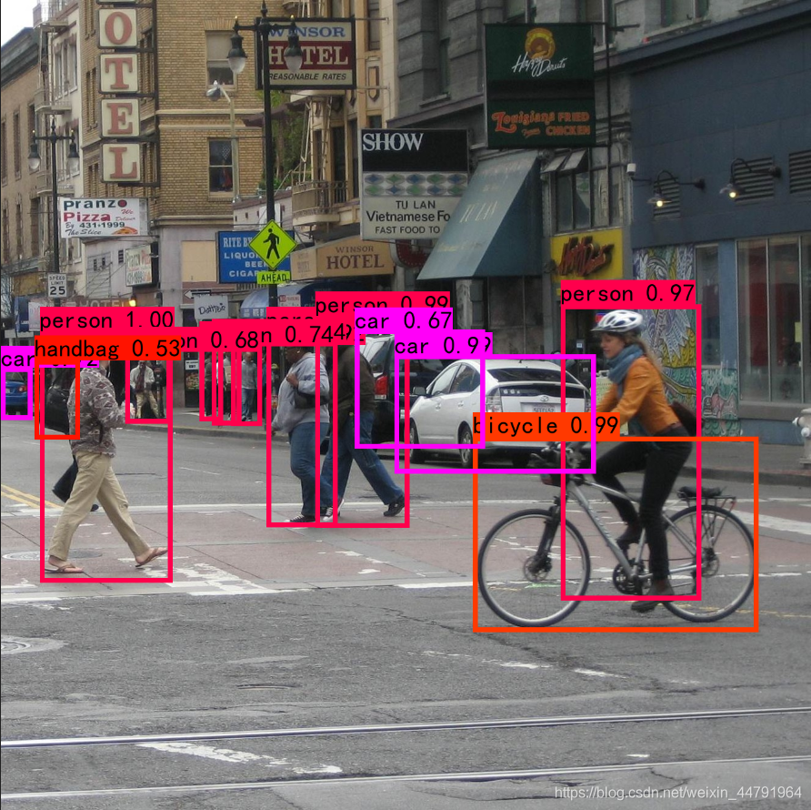
下图是未经过非极大抑制的。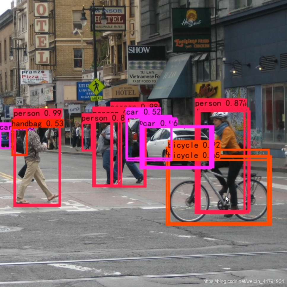
实现代码为:
defnon_max_suppression(self, prediction, num_classes, input_shape, image_shape, letterbox_image, conf_thres=0.5, nms_thres=0.4):#----------------------------------------------------------##   将预测结果的格式转换成左上角右下角的格式。#   prediction  [batch_size, num_anchors, 85]#----------------------------------------------------------#
    box_corner          = prediction.new(prediction.shape)
    box_corner[:,:,0]= prediction[:,:,0]- prediction[:,:,2]/2
    box_corner[:,:,1]= prediction[:,:,1]- prediction[:,:,3]/2
    box_corner[:,:,2]= prediction[:,:,0]+ prediction[:,:,2]/2
    box_corner[:,:,3]= prediction[:,:,1]+ prediction[:,:,3]/2
    prediction[:,:,:4]= box_corner[:,:,:4]

    output =[Nonefor _ inrange(len(prediction))]for i, image_pred inenumerate(prediction):#----------------------------------------------------------##   对种类预测部分取max。#   class_conf  [num_anchors, 1]    种类置信度#   class_pred  [num_anchors, 1]    种类#----------------------------------------------------------#
        class_conf, class_pred = torch.max(image_pred[:,5:5+ num_classes],1, keepdim=True)#----------------------------------------------------------##   利用置信度进行第一轮筛选#----------------------------------------------------------#
        conf_mask =(image_pred[:,4]* class_conf[:,0]>= conf_thres).squeeze()#----------------------------------------------------------##   根据置信度进行预测结果的筛选#----------------------------------------------------------#
        image_pred = image_pred[conf_mask]
        class_conf = class_conf[conf_mask]
        class_pred = class_pred[conf_mask]ifnot image_pred.size(0):continue#-------------------------------------------------------------------------##   detections  [num_anchors, 7]#   7的内容为:x1, y1, x2, y2, obj_conf, class_conf, class_pred#-------------------------------------------------------------------------#
        detections = torch.cat((image_pred[:,:5], class_conf.float(), class_pred.float()),1)#------------------------------------------##   获得预测结果中包含的所有种类#------------------------------------------#
        unique_labels = detections[:,-1].cpu().unique()if prediction.is_cuda:
            unique_labels = unique_labels.cuda()
            detections = detections.cuda()for c in unique_labels:#------------------------------------------##   获得某一类得分筛选后全部的预测结果#------------------------------------------#
            detections_class = detections[detections[:,-1]== c]#------------------------------------------##   使用官方自带的非极大抑制会速度更快一些!#------------------------------------------#
            keep = nms(
                detections_class[:,:4],
                detections_class[:,4]* detections_class[:,5],
                nms_thres
            )
            max_detections = detections_class[keep]# # 按照存在物体的置信度排序# _, conf_sort_index = torch.sort(detections_class[:, 4]*detections_class[:, 5], descending=True)# detections_class = detections_class[conf_sort_index]# # 进行非极大抑制# max_detections = []# while detections_class.size(0):#     # 取出这一类置信度最高的,一步一步往下判断,判断重合程度是否大于nms_thres,如果是则去除掉#     max_detections.append(detections_class[0].unsqueeze(0))#     if len(detections_class) == 1:#         break#     ious = bbox_iou(max_detections[-1], detections_class[1:])#     detections_class = detections_class[1:][ious < nms_thres]# # 堆叠# max_detections = torch.cat(max_detections).data# Add max detections to outputs
            output[i]= max_detections if output[i]isNoneelse torch.cat((output[i], max_detections))if output[i]isnotNone:
            output[i]= output[i].cpu().numpy()
            box_xy, box_wh      =(output[i][:,0:2]+ output[i][:,2:4])/2, output[i][:,2:4]- output[i][:,0:2]
            output[i][:,:4]= self.yolo_correct_boxes(box_xy, box_wh, input_shape, image_shape, letterbox_image)return output
四、训练部分
1、计算loss所需内容
计算loss实际上是网络的预测结果和网络的真实结果的对比。
和网络的预测结果一样,网络的损失也由三个部分组成,分别是Reg部分、Obj部分、Cls部分。Reg部分是特征点的回归参数判断、Obj部分是特征点是否包含物体判断、Cls部分是特征点包含的物体的种类。
2、正样本的匹配过程
在YoloV7中,训练时正样本的匹配过程可以分为两部分。
a、对每个真实框通过坐标与宽高粗略匹配先验框与特征点。
b、使用SimOTA自适应精确选取每个真实框对应多少个先验框。
所谓正样本匹配,就是寻找哪些先验框被认为有对应的真实框,并且负责这个真实框的预测。
a、匹配先验框与特征点
在该部分中,YoloV7会对每个真实框进行粗匹配。找到哪些特征点上的哪些先验框可以负责该真实框的预测。
首先进行先验框的匹配,在YoloV7网络中,一共设计了9个不同大小的先验框。每个输出的特征层对应3个先验框。
对于任何一个真实框gt,YoloV7不再使用iou进行正样本的匹配,而是直接采用高宽比进行匹配,即使用真实框和9个不同大小的先验框计算宽高比。
如果真实框与某个先验框的宽高比例大于设定阈值,则说明该真实框和该先验框匹配度不够,将该先验框认为是负样本。
比如此时有一个真实框,它的宽高为[200, 200],是一个正方形。YoloV7默认设置的9个先验框为[12, 16], [19, 36], [40, 28], [36, 75], [76, 55], [72, 146], [142, 110], [192, 243], [459, 401]。设定阈值门限为4。
此时我们需要计算该真实框和9个先验框的宽高比例。比较宽高时存在两个情况,一个是真实框的宽高比先验框大,一个是先验框的宽高比真实框大。因此我们需要同时计算:真实框的宽高/先验框的宽高;先验框的宽高/真实框的宽高。然后在这其中选取最大值。
下个列表就是比较结果,这是一个shape为[9, 4]的矩阵,9代表9个先验框,4代表真实框的宽高/先验框的宽高;先验框的宽高/真实框的宽高。
[[16.6666666712.50.060.08][10.526315795.555555560.0950.18][5.7.142857140.20.14][5.555555562.666666670.180.375][2.631578953.636363640.380.275][2.777777781.369863010.360.73][1.40845071.818181820.710.55][1.041666670.823045270.961.215][0.435729850.498753122.2952.005]]
然后对每个先验框的比较结果取最大值。获得下述矩阵:
[16.6666666710.526315797.142857145.555555563.636363642.777777781.818181821.2152.295]
之后我们判断,哪些先验框的比较结果的值小于门限。可以知道[76, 55], [72, 146], [142, 110], [192, 243], [459, 401]五个先验框均满足需求。
[142, 110], [192, 243], [459, 401]属于20,20的特征层。
[76, 55], [72, 146]属于40,40的特征层。
此时我们已经可以判断哪些大小的先验框可用于该真实框的预测。
在YoloV5过去的Yolo中,每个真实框由其中心点所在的网格内的左上角特征点来负责预测。
在YoloV7中,同YoloV5,对于被选中的特征层,首先计算真实框落在哪个网格内,此时该网格左上角特征点便是一个负责预测的特征点。
同时利用四舍五入规则,找出最近的两个网格,将这三个网格都认为是负责预测该真实框的。
红色点表示该真实框的中心,除了当前所处的网格外,其2个最近的邻域网格也被选中。从这里就可以发现预测框的XY轴偏移部分的取值范围不再是0-1,而是0.5-1.5。
找到对应特征点后,对应特征点在满足宽高比的先验框负责该真实框的预测。
但这一步仅仅是粗略的筛选,后面我们会通过simOTA来精确筛选。
deffind_3_positive(self, predictions, targets):#------------------------------------##   获得每个特征层先验框的数量#   与真实框的数量#------------------------------------#
    num_anchor, num_gt  =len(self.anchors_mask[0]), targets.shape[0]#------------------------------------##   创建空列表存放indices和anchors#------------------------------------#
    indices, anchors    =[],[]#------------------------------------##   创建7个1#   序号0,1为1#   序号2:6为特征层的高宽#   序号6为1#------------------------------------#
    gain    = torch.ones(7, device=targets.device)#------------------------------------##   ai      [num_anchor, num_gt]#   targets [num_gt, 6] => [num_anchor, num_gt, 7]#------------------------------------#
    ai      = torch.arange(num_anchor, device=targets.device).float().view(num_anchor,1).repeat(1, num_gt)
    targets = torch.cat((targets.repeat(num_anchor,1,1), ai[:,:,None]),2)# append anchor indices

    g   =0.5# offsets
    off = torch.tensor([[0,0],[1,0],[0,1],[-1,0],[0,-1],# j,k,l,m# [1, 1], [1, -1], [-1, 1], [-1, -1],  # jk,jm,lk,lm], device=targets.device).float()* g

    for i inrange(len(predictions)):#----------------------------------------------------##   将先验框除以stride,获得相对于特征层的先验框。#   anchors_i [num_anchor, 2]#----------------------------------------------------#
        anchors_i = torch.from_numpy(self.anchors[i]/ self.stride[i]).type_as(predictions[i])#-------------------------------------------##   计算获得对应特征层的高宽#-------------------------------------------#
        gain[2:6]= torch.tensor(predictions[i].shape)[[3,2,3,2]]#-------------------------------------------##   将真实框乘上gain,#   其实就是将真实框映射到特征层上#-------------------------------------------#
        t = targets * gain
        if num_gt:#-------------------------------------------##   计算真实框与先验框高宽的比值#   然后根据比值大小进行判断,#   判断结果用于取出,获得所有先验框对应的真实框#   r   [num_anchor, num_gt, 2]#   t   [num_anchor, num_gt, 7] => [num_matched_anchor, 7]#-------------------------------------------#
            r = t[:,:,4:6]/ anchors_i[:,None]
            j = torch.max(r,1./ r).max(2)[0]< self.threshold
            t = t[j]# filter#-------------------------------------------##   gxy 获得所有先验框对应的真实框的x轴y轴坐标#   gxi 取相对于该特征层的右小角的坐标#-------------------------------------------#
            gxy     = t[:,2:4]# grid xy
            gxi     = gain[[2,3]]- gxy # inverse
            j, k    =((gxy %1.< g)&(gxy >1.)).T
            l, m    =((gxi %1.< g)&(gxi >1.)).T
            j       = torch.stack((torch.ones_like(j), j, k, l, m))#-------------------------------------------##   t   重复5次,使用满足条件的j进行框的提取#   j   一共五行,代表当前特征点在五个#       [0, 0], [1, 0], [0, 1], [-1, 0], [0, -1]#       方向是否存在#-------------------------------------------#
            t       = t.repeat((5,1,1))[j]
            offsets =(torch.zeros_like(gxy)[None]+ off[:,None])[j]else:
            t = targets[0]
            offsets =0#-------------------------------------------##   b   代表属于第几个图片#   gxy 代表该真实框所处的x、y中心坐标#   gwh 代表该真实框的wh坐标#   gij 代表真实框所属的特征点坐标#-------------------------------------------#
        b, c    = t[:,:2].long().T  # image, class
        gxy     = t[:,2:4]# grid xy
        gwh     = t[:,4:6]# grid wh
        gij     =(gxy - offsets).long()
        gi, gj  = gij.T  # grid xy indices#-------------------------------------------##   gj、gi不能超出特征层范围#   a代表属于该特征点的第几个先验框#-------------------------------------------#
        a = t[:,6].long()# anchor indices
        indices.append((b, a, gj.clamp_(0, gain[3]-1), gi.clamp_(0, gain[2]-1)))# image, anchor, grid indices
        anchors.append(anchors_i[a])# anchorsreturn indices, anchors
b、SimOTA自适应匹配
在YoloV7中,我们会计算一个Cost代价矩阵,代表每个真实框和每个特征点之间的代价关系,Cost代价矩阵由三个部分组成:
1、每个真实框和当前特征点预测框的重合程度;
2、每个真实框和当前特征点预测框的种类预测准确度;
每个真实框和当前特征点预测框的重合程度越高,代表这个特征点已经尝试去拟合该真实框了,因此它的Cost代价就会越小。
每个真实框和当前特征点预测框的种类预测准确度越高,也代表这个特征点已经尝试去拟合该真实框了,因此它的Cost代价就会越小。
Cost代价矩阵的目的是自适应的找到当前特征点应该去拟合的真实框,重合度越高越需要拟合,分类越准越需要拟合,在一定半径内越需要拟合。
在SimOTA中,不同目标设定不同的正样本数量(dynamick),以旷视科技官方回答中的蚂蚁和西瓜为例子,传统的正样本分配方案常常为同一场景下的西瓜和蚂蚁分配同样的正样本数,那要么蚂蚁有很多低质量的正样本,要么西瓜仅仅只有一两个正样本。对于哪个分配方式都是不合适的。
动态的正样本设置的关键在于如何确定k,SimOTA具体的做法是首先计算每个目标Cost最低的10特征点,然后把这十个特征点对应的预测框与真实框的IOU加起来求得最终的k。
因此,SimOTA的过程总结如下:
1、计算每个真实框和当前特征点预测框的重合程度。
2、计算将重合度最高的二十个预测框与真实框的IOU加起来求得每个真实框的k,也就代表每个真实框有k个特征点与之对应。
3、计算每个真实框和当前特征点预测框的种类预测准确度。
4、计算Cost代价矩阵。
5、将Cost最低的k个点作为该真实框的正样本。
defbuild_targets(self, predictions, targets, imgs):#-------------------------------------------##   匹配正样本#-------------------------------------------#
    indices, anch       = self.find_3_positive(predictions, targets)

    matching_bs         =[[]for _ in predictions]
    matching_as         =[[]for _ in predictions]
    matching_gjs        =[[]for _ in predictions]
    matching_gis        =[[]for _ in predictions]
    matching_targets    =[[]for _ in predictions]
    matching_anchs      =[[]for _ in predictions]#-------------------------------------------##   一共三层#-------------------------------------------#
    num_layer =len(predictions)#-------------------------------------------##   对batch_size进行循环,进行OTA匹配#   在batch_size循环中对layer进行循环#-------------------------------------------#for batch_idx inrange(predictions[0].shape[0]):#-------------------------------------------##   先判断匹配上的真实框哪些属于该图片#-------------------------------------------#
        b_idx       = targets[:,0]==batch_idx
        this_target = targets[b_idx]#-------------------------------------------##   如果没有真实框属于该图片则continue#-------------------------------------------#if this_target.shape[0]==0:continue#-------------------------------------------##   真实框的坐标进行缩放#-------------------------------------------#
        txywh = this_target[:,2:6]* imgs[batch_idx].shape[1]#-------------------------------------------##   从中心宽高到左上角右下角#-------------------------------------------#
        txyxy = self.xywh2xyxy(txywh)

        pxyxys      =[]
        p_cls       =[]
        p_obj       =[]
        from_which_layer =[]
        all_b       =[]
        all_a       =[]
        all_gj      =[]
        all_gi      =[]
        all_anch    =[]#-------------------------------------------##   对三个layer进行循环#-------------------------------------------#for i, prediction inenumerate(predictions):#-------------------------------------------##   b代表第几张图片 a代表第几个先验框#   gj代表y轴,gi代表x轴#-------------------------------------------#
            b, a, gj, gi    = indices[i]
            idx             =(b == batch_idx)
            b, a, gj, gi    = b[idx], a[idx], gj[idx], gi[idx]

            all_b.append(b)
            all_a.append(a)
            all_gj.append(gj)
            all_gi.append(gi)
            all_anch.append(anch[i][idx])
            from_which_layer.append(torch.ones(size=(len(b),))* i)#-------------------------------------------##   取出这个真实框对应的预测结果#-------------------------------------------#
            fg_pred = prediction[b, a, gj, gi]
            p_obj.append(fg_pred[:,4:5])
            p_cls.append(fg_pred[:,5:])#-------------------------------------------##   获得网格后,进行解码#-------------------------------------------#
            grid    = torch.stack([gi, gj], dim=1).type_as(fg_pred)
            pxy     =(fg_pred[:,:2].sigmoid()*2.-0.5+ grid)* self.stride[i]
            pwh     =(fg_pred[:,2:4].sigmoid()*2)**2* anch[i][idx]* self.stride[i]
            pxywh   = torch.cat([pxy, pwh], dim=-1)
            pxyxy   = self.xywh2xyxy(pxywh)
            pxyxys.append(pxyxy)#-------------------------------------------##   判断是否存在对应的预测框,不存在则跳过#-------------------------------------------#
        pxyxys = torch.cat(pxyxys, dim=0)if pxyxys.shape[0]==0:continue#-------------------------------------------##   进行堆叠#-------------------------------------------#
        p_obj       = torch.cat(p_obj, dim=0)
        p_cls       = torch.cat(p_cls, dim=0)
        from_which_layer = torch.cat(from_which_layer, dim=0)
        all_b       = torch.cat(all_b, dim=0)
        all_a       = torch.cat(all_a, dim=0)
        all_gj      = torch.cat(all_gj, dim=0)
        all_gi      = torch.cat(all_gi, dim=0)
        all_anch    = torch.cat(all_anch, dim=0)#-------------------------------------------------------------##   计算当前图片中,真实框与预测框的重合程度#   iou的范围为0-1,取-log后为0~inf#   重合程度越大,取-log后越小#   因此,真实框与预测框重合度越大,pair_wise_iou_loss越小#-------------------------------------------------------------#
        pair_wise_iou       = self.box_iou(txyxy, pxyxys)
        pair_wise_iou_loss  =-torch.log(pair_wise_iou +1e-8)#-------------------------------------------##   最多二十个预测框与真实框的重合程度#   然后求和,找到每个真实框对应几个预测框#-------------------------------------------#
        top_k, _    = torch.topk(pair_wise_iou,min(20, pair_wise_iou.shape[1]), dim=1)
        dynamic_ks  = torch.clamp(top_k.sum(1).int(),min=1)#-------------------------------------------##   gt_cls_per_image    种类的真实信息#-------------------------------------------#
        gt_cls_per_image = F.one_hot(this_target[:,1].to(torch.int64), self.num_classes).float().unsqueeze(1).repeat(1, pxyxys.shape[0],1)#-------------------------------------------##   cls_preds_  种类置信度的预测信息#               cls_preds_越接近于1,y越接近于1#               y / (1 - y)越接近于无穷大#               也就是种类置信度预测的越准#               pair_wise_cls_loss越小#-------------------------------------------#
        num_gt              = this_target.shape[0]
        cls_preds_          = p_cls.float().unsqueeze(0).repeat(num_gt,1,1).sigmoid_()* p_obj.unsqueeze(0).repeat(num_gt,1,1).sigmoid_()
        y                   = cls_preds_.sqrt_()
        pair_wise_cls_loss  = F.binary_cross_entropy_with_logits(torch.log(y /(1- y)), gt_cls_per_image, reduction="none").sum(-1)del cls_preds_

        #-------------------------------------------##   求cost的总和#-------------------------------------------#
        cost =(
            pair_wise_cls_loss
            +3.0* pair_wise_iou_loss
        )#-------------------------------------------##   求cost最小的k个预测框#-------------------------------------------#
        matching_matrix = torch.zeros_like(cost)for gt_idx inrange(num_gt):
            _, pos_idx = torch.topk(cost[gt_idx], k=dynamic_ks[gt_idx].item(), largest=False)
            matching_matrix[gt_idx][pos_idx]=1.0del top_k, dynamic_ks

        #-------------------------------------------##   如果一个预测框对应多个真实框#   只使用这个预测框最对应的真实框#-------------------------------------------#
        anchor_matching_gt = matching_matrix.sum(0)if(anchor_matching_gt >1).sum()>0:
            _, cost_argmin = torch.min(cost[:, anchor_matching_gt >1], dim=0)
            matching_matrix[:, anchor_matching_gt >1]*=0.0
            matching_matrix[cost_argmin, anchor_matching_gt >1]=1.0
        fg_mask_inboxes = matching_matrix.sum(0)>0.0
        matched_gt_inds = matching_matrix[:, fg_mask_inboxes].argmax(0)#-------------------------------------------##   取出符合条件的框#-------------------------------------------#
        from_which_layer    = from_which_layer[fg_mask_inboxes]
        all_b               = all_b[fg_mask_inboxes]
        all_a               = all_a[fg_mask_inboxes]
        all_gj              = all_gj[fg_mask_inboxes]
        all_gi              = all_gi[fg_mask_inboxes]
        all_anch            = all_anch[fg_mask_inboxes]
        this_target         = this_target[matched_gt_inds]for i inrange(num_layer):
            layer_idx = from_which_layer == i
            matching_bs[i].append(all_b[layer_idx])
            matching_as[i].append(all_a[layer_idx])
            matching_gjs[i].append(all_gj[layer_idx])
            matching_gis[i].append(all_gi[layer_idx])
            matching_targets[i].append(this_target[layer_idx])
            matching_anchs[i].append(all_anch[layer_idx])for i inrange(num_layer):
        matching_bs[i]= torch.cat(matching_bs[i], dim=0)iflen(matching_bs[i])!=0else torch.Tensor(matching_bs[i])
        matching_as[i]= torch.cat(matching_as[i], dim=0)iflen(matching_as[i])!=0else torch.Tensor(matching_as[i])
        matching_gjs[i]= torch.cat(matching_gjs[i], dim=0)iflen(matching_gjs[i])!=0else torch.Tensor(matching_gjs[i])
        matching_gis[i]= torch.cat(matching_gis[i], dim=0)iflen(matching_gis[i])!=0else torch.Tensor(matching_gis[i])
        matching_targets[i]= torch.cat(matching_targets[i], dim=0)iflen(matching_targets[i])!=0else torch.Tensor(matching_targets[i])
        matching_anchs[i]= torch.cat(matching_anchs[i], dim=0)iflen(matching_anchs[i])!=0else torch.Tensor(matching_anchs[i])return matching_bs, matching_as, matching_gjs, matching_gis, matching_targets, matching_anchs
3、计算Loss
由第一部分可知,YoloV7的损失由三个部分组成:
1、Reg部分,由第2部分可知道每个真实框对应的先验框,获取到每个框对应的先验框后,取出该先验框对应的预测框,利用真实框和预测框计算CIOU损失,作为Reg部分的Loss组成。
2、Obj部分,由第2部分可知道每个真实框对应的先验框,所有真实框对应的先验框都是正样本,剩余的先验框均为负样本,根据正负样本和特征点的是否包含物体的预测结果计算交叉熵损失,作为Obj部分的Loss组成。
3、Cls部分,由第三部分可知道每个真实框对应的先验框,获取到每个框对应的先验框后,取出该先验框的种类预测结果,根据真实框的种类和先验框的种类预测结果计算交叉熵损失,作为Cls部分的Loss组成。
defsmooth_BCE(eps=0.1):# https://github.com/ultralytics/yolov3/issues/238#issuecomment-598028441# return positive, negative label smoothing BCE targetsreturn1.0-0.5* eps,0.5* eps

classYOLOLoss(nn.Module):def__init__(self, anchors, num_classes, input_shape, anchors_mask =[[6,7,8],[3,4,5],[0,1,2]], label_smoothing =0):super(YOLOLoss, self).__init__()#-----------------------------------------------------------##   13x13的特征层对应的anchor是[142, 110],[192, 243],[459, 401]#   26x26的特征层对应的anchor是[36, 75],[76, 55],[72, 146]#   52x52的特征层对应的anchor是[12, 16],[19, 36],[40, 28]#-----------------------------------------------------------#
        self.anchors        =[anchors[mask]for mask in anchors_mask]
        self.num_classes    = num_classes
        self.input_shape    = input_shape
        self.anchors_mask   = anchors_mask

        self.balance        =[0.4,1.0,4]
        self.stride         =[32,16,8]

        self.box_ratio      =0.05
        self.obj_ratio      =1*(input_shape[0]* input_shape[1])/(640**2)
        self.cls_ratio      =0.5*(num_classes /80)
        self.threshold      =4

        self.cp, self.cn                    = smooth_BCE(eps=label_smoothing)
        self.BCEcls, self.BCEobj, self.gr   = nn.BCEWithLogitsLoss(), nn.BCEWithLogitsLoss(),1defbbox_iou(self, box1, box2, x1y1x2y2=True, GIoU=False, DIoU=False, CIoU=False, eps=1e-7):
        box2 = box2.T

        if x1y1x2y2:
            b1_x1, b1_y1, b1_x2, b1_y2 = box1[0], box1[1], box1[2], box1[3]
            b2_x1, b2_y1, b2_x2, b2_y2 = box2[0], box2[1], box2[2], box2[3]else:
            b1_x1, b1_x2 = box1[0]- box1[2]/2, box1[0]+ box1[2]/2
            b1_y1, b1_y2 = box1[1]- box1[3]/2, box1[1]+ box1[3]/2
            b2_x1, b2_x2 = box2[0]- box2[2]/2, box2[0]+ box2[2]/2
            b2_y1, b2_y2 = box2[1]- box2[3]/2, box2[1]+ box2[3]/2

        inter =(torch.min(b1_x2, b2_x2)- torch.max(b1_x1, b2_x1)).clamp(0)* \
                (torch.min(b1_y2, b2_y2)- torch.max(b1_y1, b2_y1)).clamp(0)

        w1, h1  = b1_x2 - b1_x1, b1_y2 - b1_y1 + eps
        w2, h2  = b2_x2 - b2_x1, b2_y2 - b2_y1 + eps
        union   = w1 * h1 + w2 * h2 - inter + eps

        iou = inter / union

        if GIoU or DIoU or CIoU:
            cw = torch.max(b1_x2, b2_x2)- torch.min(b1_x1, b2_x1)# convex (smallest enclosing box) width
            ch = torch.max(b1_y2, b2_y2)- torch.min(b1_y1, b2_y1)# convex heightif CIoU or DIoU:# Distance or Complete IoU https://arxiv.org/abs/1911.08287v1
                c2 = cw **2+ ch **2+ eps  # convex diagonal squared
                rho2 =((b2_x1 + b2_x2 - b1_x1 - b1_x2)**2+(b2_y1 + b2_y2 - b1_y1 - b1_y2)**2)/4# center distance squaredif DIoU:return iou - rho2 / c2  # DIoUelif CIoU:# https://github.com/Zzh-tju/DIoU-SSD-pytorch/blob/master/utils/box/box_utils.py#L47
                    v =(4/ math.pi **2)* torch.pow(torch.atan(w2 / h2)- torch.atan(w1 / h1),2)with torch.no_grad():
                        alpha = v /(v - iou +(1+ eps))return iou -(rho2 / c2 + v * alpha)# CIoUelse:# GIoU https://arxiv.org/pdf/1902.09630.pdf
                c_area = cw * ch + eps  # convex areareturn iou -(c_area - union)/ c_area  # GIoUelse:return iou  # IoUdef__call__(self, predictions, targets, imgs):#-------------------------------------------##   对输入进来的预测结果进行reshape#   bs, 255, 20, 20 => bs, 3, 20, 20, 85#   bs, 255, 40, 40 => bs, 3, 40, 40, 85#   bs, 255, 80, 80 => bs, 3, 80, 80, 85#-------------------------------------------#for i inrange(len(predictions)):
            bs, _, h, w = predictions[i].size()
            predictions[i]= predictions[i].view(bs,len(self.anchors_mask[i]),-1, h, w).permute(0,1,3,4,2).contiguous()#-------------------------------------------##   获得工作的设备#-------------------------------------------#
        device              = targets.device
        #-------------------------------------------##   初始化三个部分的损失#-------------------------------------------#
        cls_loss, box_loss, obj_loss    = torch.zeros(1, device = device), torch.zeros(1, device = device), torch.zeros(1, device = device)#-------------------------------------------##   进行正样本的匹配#-------------------------------------------#
        bs, as_, gjs, gis, targets, anchors = self.build_targets(predictions, targets, imgs)#-------------------------------------------##   计算获得对应特征层的高宽#-------------------------------------------#
        feature_map_sizes =[torch.tensor(prediction.shape, device=device)[[3,2,3,2]].type_as(prediction)for prediction in predictions]#-------------------------------------------##   计算损失,对三个特征层各自进行处理#-------------------------------------------#for i, prediction inenumerate(predictions):#-------------------------------------------##   image, anchor, gridy, gridx#-------------------------------------------#
            b, a, gj, gi    = bs[i], as_[i], gjs[i], gis[i]
            tobj            = torch.zeros_like(prediction[...,0], device=device)# target obj#-------------------------------------------##   获得目标数量,如果目标大于0#   则开始计算种类损失和回归损失#-------------------------------------------#
            n = b.shape[0]if n:
                prediction_pos = prediction[b, a, gj, gi]# prediction subset corresponding to targets#-------------------------------------------##   计算匹配上的正样本的回归损失#-------------------------------------------##-------------------------------------------##   grid 获得正样本的x、y轴坐标#-------------------------------------------#
                grid    = torch.stack([gi, gj], dim=1)#-------------------------------------------##   进行解码,获得预测结果#-------------------------------------------#
                xy      = prediction_pos[:,:2].sigmoid()*2.-0.5
                wh      =(prediction_pos[:,2:4].sigmoid()*2)**2* anchors[i]
                box     = torch.cat((xy, wh),1)#-------------------------------------------##   对真实框进行处理,映射到特征层上#-------------------------------------------#
                selected_tbox           = targets[i][:,2:6]* feature_map_sizes[i]
                selected_tbox[:,:2]-= grid.type_as(prediction)#-------------------------------------------##   计算预测框和真实框的回归损失#-------------------------------------------#
                iou                     = self.bbox_iou(box.T, selected_tbox, x1y1x2y2=False, CIoU=True)
                box_loss                +=(1.0- iou).mean()#-------------------------------------------##   根据预测结果的iou获得置信度损失的gt#-------------------------------------------#
                tobj[b, a, gj, gi]=(1.0- self.gr)+ self.gr * iou.detach().clamp(0).type(tobj.dtype)# iou ratio#-------------------------------------------##   计算匹配上的正样本的分类损失#-------------------------------------------#
                selected_tcls               = targets[i][:,1].long()
                t                           = torch.full_like(prediction_pos[:,5:], self.cn, device=device)# targets
                t[range(n), selected_tcls]= self.cp
                cls_loss                    += self.BCEcls(prediction_pos[:,5:], t)# BCE#-------------------------------------------##   计算目标是否存在的置信度损失#   并且乘上每个特征层的比例#-------------------------------------------#
            obj_loss += self.BCEobj(prediction[...,4], tobj)* self.balance[i]# obj loss#-------------------------------------------##   将各个部分的损失乘上比例#   全加起来后,乘上batch_size#-------------------------------------------#
        box_loss    *= self.box_ratio
        obj_loss    *= self.obj_ratio
        cls_loss    *= self.cls_ratio
        bs          = tobj.shape[0]

        loss    = box_loss + obj_loss + cls_loss
        return loss

    defxywh2xyxy(self, x):# Convert nx4 boxes from [x, y, w, h] to [x1, y1, x2, y2]
        y = x.clone()ifisinstance(x, torch.Tensor)else np.copy(x)
        y[:,0]= x[:,0]- x[:,2]/2# top left x
        y[:,1]= x[:,1]- x[:,3]/2# top left y
        y[:,2]= x[:,0]+ x[:,2]/2# bottom right x
        y[:,3]= x[:,1]+ x[:,3]/2# bottom right yreturn y

    defbox_iou(self, box1, box2):# https://github.com/pytorch/vision/blob/master/torchvision/ops/boxes.py"""
        Return intersection-over-union (Jaccard index) of boxes.
        Both sets of boxes are expected to be in (x1, y1, x2, y2) format.
        Arguments:
            box1 (Tensor[N, 4])
            box2 (Tensor[M, 4])
        Returns:
            iou (Tensor[N, M]): the NxM matrix containing the pairwise
                IoU values for every element in boxes1 and boxes2
        """defbox_area(box):# box = 4xnreturn(box[2]- box[0])*(box[3]- box[1])

        area1 = box_area(box1.T)
        area2 = box_area(box2.T)# inter(N,M) = (rb(N,M,2) - lt(N,M,2)).clamp(0).prod(2)
        inter =(torch.min(box1[:,None,2:], box2[:,2:])- torch.max(box1[:,None,:2], box2[:,:2])).clamp(0).prod(2)return inter /(area1[:,None]+ area2 - inter)# iou = inter / (area1 + area2 - inter)defbuild_targets(self, predictions, targets, imgs):#-------------------------------------------##   匹配正样本#-------------------------------------------#
        indices, anch       = self.find_3_positive(predictions, targets)

        matching_bs         =[[]for _ in predictions]
        matching_as         =[[]for _ in predictions]
        matching_gjs        =[[]for _ in predictions]
        matching_gis        =[[]for _ in predictions]
        matching_targets    =[[]for _ in predictions]
        matching_anchs      =[[]for _ in predictions]#-------------------------------------------##   一共三层#-------------------------------------------#
        num_layer =len(predictions)#-------------------------------------------##   对batch_size进行循环,进行OTA匹配#   在batch_size循环中对layer进行循环#-------------------------------------------#for batch_idx inrange(predictions[0].shape[0]):#-------------------------------------------##   先判断匹配上的真实框哪些属于该图片#-------------------------------------------#
            b_idx       = targets[:,0]==batch_idx
            this_target = targets[b_idx]#-------------------------------------------##   如果没有真实框属于该图片则continue#-------------------------------------------#if this_target.shape[0]==0:continue#-------------------------------------------##   真实框的坐标进行缩放#-------------------------------------------#
            txywh = this_target[:,2:6]* imgs[batch_idx].shape[1]#-------------------------------------------##   从中心宽高到左上角右下角#-------------------------------------------#
            txyxy = self.xywh2xyxy(txywh)

            pxyxys      =[]
            p_cls       =[]
            p_obj       =[]
            from_which_layer =[]
            all_b       =[]
            all_a       =[]
            all_gj      =[]
            all_gi      =[]
            all_anch    =[]#-------------------------------------------##   对三个layer进行循环#-------------------------------------------#for i, prediction inenumerate(predictions):#-------------------------------------------##   b代表第几张图片 a代表第几个先验框#   gj代表y轴,gi代表x轴#-------------------------------------------#
                b, a, gj, gi    = indices[i]
                idx             =(b == batch_idx)
                b, a, gj, gi    = b[idx], a[idx], gj[idx], gi[idx]

                all_b.append(b)
                all_a.append(a)
                all_gj.append(gj)
                all_gi.append(gi)
                all_anch.append(anch[i][idx])
                from_which_layer.append(torch.ones(size=(len(b),))* i)#-------------------------------------------##   取出这个真实框对应的预测结果#-------------------------------------------#
                fg_pred = prediction[b, a, gj, gi]
                p_obj.append(fg_pred[:,4:5])
                p_cls.append(fg_pred[:,5:])#-------------------------------------------##   获得网格后,进行解码#-------------------------------------------#
                grid    = torch.stack([gi, gj], dim=1).type_as(fg_pred)
                pxy     =(fg_pred[:,:2].sigmoid()*2.-0.5+ grid)* self.stride[i]
                pwh     =(fg_pred[:,2:4].sigmoid()*2)**2* anch[i][idx]* self.stride[i]
                pxywh   = torch.cat([pxy, pwh], dim=-1)
                pxyxy   = self.xywh2xyxy(pxywh)
                pxyxys.append(pxyxy)#-------------------------------------------##   判断是否存在对应的预测框,不存在则跳过#-------------------------------------------#
            pxyxys = torch.cat(pxyxys, dim=0)if pxyxys.shape[0]==0:continue#-------------------------------------------##   进行堆叠#-------------------------------------------#
            p_obj       = torch.cat(p_obj, dim=0)
            p_cls       = torch.cat(p_cls, dim=0)
            from_which_layer = torch.cat(from_which_layer, dim=0)
            all_b       = torch.cat(all_b, dim=0)
            all_a       = torch.cat(all_a, dim=0)
            all_gj      = torch.cat(all_gj, dim=0)
            all_gi      = torch.cat(all_gi, dim=0)
            all_anch    = torch.cat(all_anch, dim=0)#-------------------------------------------------------------##   计算当前图片中,真实框与预测框的重合程度#   iou的范围为0-1,取-log后为0~inf#   重合程度越大,取-log后越小#   因此,真实框与预测框重合度越大,pair_wise_iou_loss越小#-------------------------------------------------------------#
            pair_wise_iou       = self.box_iou(txyxy, pxyxys)
            pair_wise_iou_loss  =-torch.log(pair_wise_iou +1e-8)#-------------------------------------------##   最多二十个预测框与真实框的重合程度#   然后求和,找到每个真实框对应几个预测框#-------------------------------------------#
            top_k, _    = torch.topk(pair_wise_iou,min(20, pair_wise_iou.shape[1]), dim=1)
            dynamic_ks  = torch.clamp(top_k.sum(1).int(),min=1)#-------------------------------------------##   gt_cls_per_image    种类的真实信息#-------------------------------------------#
            gt_cls_per_image = F.one_hot(this_target[:,1].to(torch.int64), self.num_classes).float().unsqueeze(1).repeat(1, pxyxys.shape[0],1)#-------------------------------------------##   cls_preds_  种类置信度的预测信息#               cls_preds_越接近于1,y越接近于1#               y / (1 - y)越接近于无穷大#               也就是种类置信度预测的越准#               pair_wise_cls_loss越小#-------------------------------------------#
            num_gt              = this_target.shape[0]
            cls_preds_          = p_cls.float().unsqueeze(0).repeat(num_gt,1,1).sigmoid_()* p_obj.unsqueeze(0).repeat(num_gt,1,1).sigmoid_()
            y                   = cls_preds_.sqrt_()
            pair_wise_cls_loss  = F.binary_cross_entropy_with_logits(torch.log(y /(1- y)), gt_cls_per_image, reduction="none").sum(-1)del cls_preds_

            #-------------------------------------------##   求cost的总和#-------------------------------------------#
            cost =(
                pair_wise_cls_loss
                +3.0* pair_wise_iou_loss
            )#-------------------------------------------##   求cost最小的k个预测框#-------------------------------------------#
            matching_matrix = torch.zeros_like(cost)for gt_idx inrange(num_gt):
                _, pos_idx = torch.topk(cost[gt_idx], k=dynamic_ks[gt_idx].item(), largest=False)
                matching_matrix[gt_idx][pos_idx]=1.0del top_k, dynamic_ks

            #-------------------------------------------##   如果一个预测框对应多个真实框#   只使用这个预测框最对应的真实框#-------------------------------------------#
            anchor_matching_gt = matching_matrix.sum(0)if(anchor_matching_gt >1).sum()>0:
                _, cost_argmin = torch.min(cost[:, anchor_matching_gt >1], dim=0)
                matching_matrix[:, anchor_matching_gt >1]*=0.0
                matching_matrix[cost_argmin, anchor_matching_gt >1]=1.0
            fg_mask_inboxes = matching_matrix.sum(0)>0.0
            matched_gt_inds = matching_matrix[:, fg_mask_inboxes].argmax(0)#-------------------------------------------##   取出符合条件的框#-------------------------------------------#
            from_which_layer    = from_which_layer[fg_mask_inboxes]
            all_b               = all_b[fg_mask_inboxes]
            all_a               = all_a[fg_mask_inboxes]
            all_gj              = all_gj[fg_mask_inboxes]
            all_gi              = all_gi[fg_mask_inboxes]
            all_anch            = all_anch[fg_mask_inboxes]
            this_target         = this_target[matched_gt_inds]for i inrange(num_layer):
                layer_idx = from_which_layer == i
                matching_bs[i].append(all_b[layer_idx])
                matching_as[i].append(all_a[layer_idx])
                matching_gjs[i].append(all_gj[layer_idx])
                matching_gis[i].append(all_gi[layer_idx])
                matching_targets[i].append(this_target[layer_idx])
                matching_anchs[i].append(all_anch[layer_idx])for i inrange(num_layer):
            matching_bs[i]= torch.cat(matching_bs[i], dim=0)iflen(matching_bs[i])!=0else torch.Tensor(matching_bs[i])
            matching_as[i]= torch.cat(matching_as[i], dim=0)iflen(matching_as[i])!=0else torch.Tensor(matching_as[i])
            matching_gjs[i]= torch.cat(matching_gjs[i], dim=0)iflen(matching_gjs[i])!=0else torch.Tensor(matching_gjs[i])
            matching_gis[i]= torch.cat(matching_gis[i], dim=0)iflen(matching_gis[i])!=0else torch.Tensor(matching_gis[i])
            matching_targets[i]= torch.cat(matching_targets[i], dim=0)iflen(matching_targets[i])!=0else torch.Tensor(matching_targets[i])
            matching_anchs[i]= torch.cat(matching_anchs[i], dim=0)iflen(matching_anchs[i])!=0else torch.Tensor(matching_anchs[i])return matching_bs, matching_as, matching_gjs, matching_gis, matching_targets, matching_anchs

    deffind_3_positive(self, predictions, targets):#------------------------------------##   获得每个特征层先验框的数量#   与真实框的数量#------------------------------------#
        num_anchor, num_gt  =len(self.anchors_mask[0]), targets.shape[0]#------------------------------------##   创建空列表存放indices和anchors#------------------------------------#
        indices, anchors    =[],[]#------------------------------------##   创建7个1#   序号0,1为1#   序号2:6为特征层的高宽#   序号6为1#------------------------------------#
        gain    = torch.ones(7, device=targets.device)#------------------------------------##   ai      [num_anchor, num_gt]#   targets [num_gt, 6] => [num_anchor, num_gt, 7]#------------------------------------#
        ai      = torch.arange(num_anchor, device=targets.device).float().view(num_anchor,1).repeat(1, num_gt)
        targets = torch.cat((targets.repeat(num_anchor,1,1), ai[:,:,None]),2)# append anchor indices

        g   =0.5# offsets
        off = torch.tensor([[0,0],[1,0],[0,1],[-1,0],[0,-1],# j,k,l,m# [1, 1], [1, -1], [-1, 1], [-1, -1],  # jk,jm,lk,lm], device=targets.device).float()* g

        for i inrange(len(predictions)):#----------------------------------------------------##   将先验框除以stride,获得相对于特征层的先验框。#   anchors_i [num_anchor, 2]#----------------------------------------------------#
            anchors_i = torch.from_numpy(self.anchors[i]/ self.stride[i]).type_as(predictions[i])#-------------------------------------------##   计算获得对应特征层的高宽#-------------------------------------------#
            gain[2:6]= torch.tensor(predictions[i].shape)[[3,2,3,2]]#-------------------------------------------##   将真实框乘上gain,#   其实就是将真实框映射到特征层上#-------------------------------------------#
            t = targets * gain
            if num_gt:#-------------------------------------------##   计算真实框与先验框高宽的比值#   然后根据比值大小进行判断,#   判断结果用于取出,获得所有先验框对应的真实框#   r   [num_anchor, num_gt, 2]#   t   [num_anchor, num_gt, 7] => [num_matched_anchor, 7]#-------------------------------------------#
                r = t[:,:,4:6]/ anchors_i[:,None]
                j = torch.max(r,1./ r).max(2)[0]< self.threshold
                t = t[j]# filter#-------------------------------------------##   gxy 获得所有先验框对应的真实框的x轴y轴坐标#   gxi 取相对于该特征层的右小角的坐标#-------------------------------------------#
                gxy     = t[:,2:4]# grid xy
                gxi     = gain[[2,3]]- gxy # inverse
                j, k    =((gxy %1.< g)&(gxy >1.)).T
                l, m    =((gxi %1.< g)&(gxi >1.)).T
                j       = torch.stack((torch.ones_like(j), j, k, l, m))#-------------------------------------------##   t   重复5次,使用满足条件的j进行框的提取#   j   一共五行,代表当前特征点在五个#       [0, 0], [1, 0], [0, 1], [-1, 0], [0, -1]#       方向是否存在#-------------------------------------------#
                t       = t.repeat((5,1,1))[j]
                offsets =(torch.zeros_like(gxy)[None]+ off[:,None])[j]else:
                t = targets[0]
                offsets =0#-------------------------------------------##   b   代表属于第几个图片#   gxy 代表该真实框所处的x、y中心坐标#   gwh 代表该真实框的wh坐标#   gij 代表真实框所属的特征点坐标#-------------------------------------------#
            b, c    = t[:,:2].long().T  # image, class
            gxy     = t[:,2:4]# grid xy
            gwh     = t[:,4:6]# grid wh
            gij     =(gxy - offsets).long()
            gi, gj  = gij.T  # grid xy indices#-------------------------------------------##   gj、gi不能超出特征层范围#   a代表属于该特征点的第几个先验框#-------------------------------------------#
            a = t[:,6].long()# anchor indices
            indices.append((b, a, gj.clamp_(0, gain[3]-1), gi.clamp_(0, gain[2]-1)))# image, anchor, grid indices
            anchors.append(anchors_i[a])# anchorsreturn indices, anchors
训练自己的YoloV7模型
首先前往Github下载对应的仓库,下载完后利用解压软件解压,之后用编程软件打开文件夹。
注意打开的根目录必须正确,否则相对目录不正确的情况下,代码将无法运行。
一定要注意打开后的根目录是文件存放的目录。
一、数据集的准备
本文使用VOC格式进行训练,训练前需要自己制作好数据集,如果没有自己的数据集,可以通过Github连接下载VOC12+07的数据集尝试下。
训练前将标签文件放在VOCdevkit文件夹下的VOC2007文件夹下的Annotation中。
训练前将图片文件放在VOCdevkit文件夹下的VOC2007文件夹下的JPEGImages中。
此时数据集的摆放已经结束。
二、数据集的处理
在完成数据集的摆放之后,我们需要对数据集进行下一步的处理,目的是获得训练用的2007_train.txt以及2007_val.txt,需要用到根目录下的voc_annotation.py。
voc_annotation.py里面有一些参数需要设置。
分别是annotation_mode、classes_path、trainval_percent、train_percent、VOCdevkit_path,第一次训练可以仅修改classes_path
'''
annotation_mode用于指定该文件运行时计算的内容
annotation_mode为0代表整个标签处理过程,包括获得VOCdevkit/VOC2007/ImageSets里面的txt以及训练用的2007_train.txt、2007_val.txt
annotation_mode为1代表获得VOCdevkit/VOC2007/ImageSets里面的txt
annotation_mode为2代表获得训练用的2007_train.txt、2007_val.txt
'''
annotation_mode     =0'''
必须要修改,用于生成2007_train.txt、2007_val.txt的目标信息
与训练和预测所用的classes_path一致即可
如果生成的2007_train.txt里面没有目标信息
那么就是因为classes没有设定正确
仅在annotation_mode为0和2的时候有效
'''
classes_path        ='model_data/voc_classes.txt''''
trainval_percent用于指定(训练集+验证集)与测试集的比例,默认情况下 (训练集+验证集):测试集 = 9:1
train_percent用于指定(训练集+验证集)中训练集与验证集的比例,默认情况下 训练集:验证集 = 9:1
仅在annotation_mode为0和1的时候有效
'''
trainval_percent    =0.9
train_percent       =0.9'''
指向VOC数据集所在的文件夹
默认指向根目录下的VOC数据集
'''
VOCdevkit_path  ='VOCdevkit'
classes_path用于指向检测类别所对应的txt,以voc数据集为例,我们用的txt为:
训练自己的数据集时,可以自己建立一个cls_classes.txt,里面写自己所需要区分的类别。
三、开始网络训练
通过voc_annotation.py我们已经生成了2007_train.txt以及2007_val.txt,此时我们可以开始训练了。
训练的参数较多,大家可以在下载库后仔细看注释,其中最重要的部分依然是train.py里的classes_path。
classes_path用于指向检测类别所对应的txt,这个txt和voc_annotation.py里面的txt一样!训练自己的数据集必须要修改!
修改完classes_path后就可以运行train.py开始训练了,在训练多个epoch后,权值会生成在logs文件夹中。
其它参数的作用如下:
#---------------------------------##   Cuda    是否使用Cuda#           没有GPU可以设置成False#---------------------------------#
Cuda            =True#---------------------------------------------------------------------##   distributed     用于指定是否使用单机多卡分布式运行#                   终端指令仅支持Ubuntu。CUDA_VISIBLE_DEVICES用于在Ubuntu下指定显卡。#                   Windows系统下默认使用DP模式调用所有显卡,不支持DDP。#   DP模式:#       设置            distributed = False#       在终端中输入    CUDA_VISIBLE_DEVICES=0,1 python train.py#   DDP模式:#       设置            distributed = True#       在终端中输入    CUDA_VISIBLE_DEVICES=0,1 python -m torch.distributed.launch --nproc_per_node=2 train.py#---------------------------------------------------------------------#
distributed     =False#---------------------------------------------------------------------##   sync_bn     是否使用sync_bn,DDP模式多卡可用#---------------------------------------------------------------------#
sync_bn         =False#---------------------------------------------------------------------##   fp16        是否使用混合精度训练#               可减少约一半的显存、需要pytorch1.7.1以上#---------------------------------------------------------------------#
fp16            =False#---------------------------------------------------------------------##   classes_path    指向model_data下的txt,与自己训练的数据集相关 #                   训练前一定要修改classes_path,使其对应自己的数据集#---------------------------------------------------------------------#
classes_path    ='model_data/voc_classes.txt'#---------------------------------------------------------------------##   anchors_path    代表先验框对应的txt文件,一般不修改。#   anchors_mask    用于帮助代码找到对应的先验框,一般不修改。#---------------------------------------------------------------------#
anchors_path    ='model_data/yolo_anchors.txt'
anchors_mask    =[[6,7,8],[3,4,5],[0,1,2]]#----------------------------------------------------------------------------------------------------------------------------##   权值文件的下载请看README,可以通过网盘下载。模型的 预训练权重 对不同数据集是通用的,因为特征是通用的。#   模型的 预训练权重 比较重要的部分是 主干特征提取网络的权值部分,用于进行特征提取。#   预训练权重对于99%的情况都必须要用,不用的话主干部分的权值太过随机,特征提取效果不明显,网络训练的结果也不会好##   如果训练过程中存在中断训练的操作,可以将model_path设置成logs文件夹下的权值文件,将已经训练了一部分的权值再次载入。#   同时修改下方的 冻结阶段 或者 解冻阶段 的参数,来保证模型epoch的连续性。#   #   当model_path = ''的时候不加载整个模型的权值。##   此处使用的是整个模型的权重,因此是在train.py进行加载的。#   如果想要让模型从0开始训练,则设置model_path = '',下面的Freeze_Train = Fasle,此时从0开始训练,且没有冻结主干的过程。#   #   一般来讲,网络从0开始的训练效果会很差,因为权值太过随机,特征提取效果不明显,因此非常、非常、非常不建议大家从0开始训练!#   从0开始训练有两个方案:#   1、得益于Mosaic数据增强方法强大的数据增强能力,将UnFreeze_Epoch设置的较大(300及以上)、batch较大(16及以上)、数据较多(万以上)的情况下,#      可以设置mosaic=True,直接随机初始化参数开始训练,但得到的效果仍然不如有预训练的情况。(像COCO这样的大数据集可以这样做)#   2、了解imagenet数据集,首先训练分类模型,获得网络的主干部分权值,分类模型的 主干部分 和该模型通用,基于此进行训练。#----------------------------------------------------------------------------------------------------------------------------#
model_path      ='model_data/yolov7_weights.pth'#------------------------------------------------------##   input_shape     输入的shape大小,一定要是32的倍数#------------------------------------------------------#
input_shape     =[640,640]#------------------------------------------------------##   phi             所使用到的yolov7的版本,本仓库一共提供两个:#                   l : 对应yolov7#                   x : 对应yolov7_x#------------------------------------------------------#
phi             ='l'#----------------------------------------------------------------------------------------------------------------------------##   pretrained      是否使用主干网络的预训练权重,此处使用的是主干的权重,因此是在模型构建的时候进行加载的。#                   如果设置了model_path,则主干的权值无需加载,pretrained的值无意义。#                   如果不设置model_path,pretrained = True,此时仅加载主干开始训练。#                   如果不设置model_path,pretrained = False,Freeze_Train = Fasle,此时从0开始训练,且没有冻结主干的过程。#----------------------------------------------------------------------------------------------------------------------------#
pretrained      =False#------------------------------------------------------------------##   mosaic              马赛克数据增强。#   mosaic_prob         每个step有多少概率使用mosaic数据增强,默认50%。##   mixup               是否使用mixup数据增强,仅在mosaic=True时有效。#                       只会对mosaic增强后的图片进行mixup的处理。#   mixup_prob          有多少概率在mosaic后使用mixup数据增强,默认50%。#                       总的mixup概率为mosaic_prob * mixup_prob。##   special_aug_ratio   参考YoloX,由于Mosaic生成的训练图片,远远脱离自然图片的真实分布。#                       当mosaic=True时,本代码会在special_aug_ratio范围内开启mosaic。#                       默认为前70%个epoch,100个世代会开启70个世代。#------------------------------------------------------------------#
mosaic              =True
mosaic_prob         =0.5
mixup               =True
mixup_prob          =0.5
special_aug_ratio   =0.7#------------------------------------------------------------------##   label_smoothing     标签平滑。一般0.01以下。如0.01、0.005。#------------------------------------------------------------------#
label_smoothing     =0#----------------------------------------------------------------------------------------------------------------------------##   训练分为两个阶段,分别是冻结阶段和解冻阶段。设置冻结阶段是为了满足机器性能不足的同学的训练需求。#   冻结训练需要的显存较小,显卡非常差的情况下,可设置Freeze_Epoch等于UnFreeze_Epoch,Freeze_Train = True,此时仅仅进行冻结训练。#      #   在此提供若干参数设置建议,各位训练者根据自己的需求进行灵活调整:#   (一)从整个模型的预训练权重开始训练: #       Adam:#           Init_Epoch = 0,Freeze_Epoch = 50,UnFreeze_Epoch = 100,Freeze_Train = True,optimizer_type = 'adam',Init_lr = 1e-3,weight_decay = 0。(冻结)#           Init_Epoch = 0,UnFreeze_Epoch = 100,Freeze_Train = False,optimizer_type = 'adam',Init_lr = 1e-3,weight_decay = 0。(不冻结)#       SGD:#           Init_Epoch = 0,Freeze_Epoch = 50,UnFreeze_Epoch = 300,Freeze_Train = True,optimizer_type = 'sgd',Init_lr = 1e-2,weight_decay = 5e-4。(冻结)#           Init_Epoch = 0,UnFreeze_Epoch = 300,Freeze_Train = False,optimizer_type = 'sgd',Init_lr = 1e-2,weight_decay = 5e-4。(不冻结)#       其中:UnFreeze_Epoch可以在100-300之间调整。#   (二)从0开始训练:#       Init_Epoch = 0,UnFreeze_Epoch >= 300,Unfreeze_batch_size >= 16,Freeze_Train = False(不冻结训练)#       其中:UnFreeze_Epoch尽量不小于300。optimizer_type = 'sgd',Init_lr = 1e-2,mosaic = True。#   (三)batch_size的设置:#       在显卡能够接受的范围内,以大为好。显存不足与数据集大小无关,提示显存不足(OOM或者CUDA out of memory)请调小batch_size。#       受到BatchNorm层影响,batch_size最小为2,不能为1。#       正常情况下Freeze_batch_size建议为Unfreeze_batch_size的1-2倍。不建议设置的差距过大,因为关系到学习率的自动调整。#----------------------------------------------------------------------------------------------------------------------------##------------------------------------------------------------------##   冻结阶段训练参数#   此时模型的主干被冻结了,特征提取网络不发生改变#   占用的显存较小,仅对网络进行微调#   Init_Epoch          模型当前开始的训练世代,其值可以大于Freeze_Epoch,如设置:#                       Init_Epoch = 60、Freeze_Epoch = 50、UnFreeze_Epoch = 100#                       会跳过冻结阶段,直接从60代开始,并调整对应的学习率。#                       (断点续练时使用)#   Freeze_Epoch        模型冻结训练的Freeze_Epoch#                       (当Freeze_Train=False时失效)#   Freeze_batch_size   模型冻结训练的batch_size#                       (当Freeze_Train=False时失效)#------------------------------------------------------------------#
Init_Epoch          =0
Freeze_Epoch        =50
Freeze_batch_size   =8#------------------------------------------------------------------##   解冻阶段训练参数#   此时模型的主干不被冻结了,特征提取网络会发生改变#   占用的显存较大,网络所有的参数都会发生改变#   UnFreeze_Epoch          模型总共训练的epoch#                           SGD需要更长的时间收敛,因此设置较大的UnFreeze_Epoch#                           Adam可以使用相对较小的UnFreeze_Epoch#   Unfreeze_batch_size     模型在解冻后的batch_size#------------------------------------------------------------------#
UnFreeze_Epoch      =300
Unfreeze_batch_size =4#------------------------------------------------------------------##   Freeze_Train    是否进行冻结训练#                   默认先冻结主干训练后解冻训练。#------------------------------------------------------------------#
Freeze_Train        =True#------------------------------------------------------------------##   其它训练参数:学习率、优化器、学习率下降有关#------------------------------------------------------------------##------------------------------------------------------------------##   Init_lr         模型的最大学习率#   Min_lr          模型的最小学习率,默认为最大学习率的0.01#------------------------------------------------------------------#
Init_lr             =1e-2
Min_lr              = Init_lr *0.01#------------------------------------------------------------------##   optimizer_type  使用到的优化器种类,可选的有adam、sgd#                   当使用Adam优化器时建议设置  Init_lr=1e-3#                   当使用SGD优化器时建议设置   Init_lr=1e-2#   momentum        优化器内部使用到的momentum参数#   weight_decay    权值衰减,可防止过拟合#                   adam会导致weight_decay错误,使用adam时建议设置为0。#------------------------------------------------------------------#
optimizer_type      ="sgd"
momentum            =0.937
weight_decay        =5e-4#------------------------------------------------------------------##   lr_decay_type   使用到的学习率下降方式,可选的有step、cos#------------------------------------------------------------------#
lr_decay_type       ="cos"#------------------------------------------------------------------##   save_period     多少个epoch保存一次权值#------------------------------------------------------------------#
save_period         =10#------------------------------------------------------------------##   save_dir        权值与日志文件保存的文件夹#------------------------------------------------------------------#
save_dir            ='logs'#------------------------------------------------------------------##   eval_flag       是否在训练时进行评估,评估对象为验证集#                   安装pycocotools库后,评估体验更佳。#   eval_period     代表多少个epoch评估一次,不建议频繁的评估#                   评估需要消耗较多的时间,频繁评估会导致训练非常慢#   此处获得的mAP会与get_map.py获得的会有所不同,原因有二:#   (一)此处获得的mAP为验证集的mAP。#   (二)此处设置评估参数较为保守,目的是加快评估速度。#------------------------------------------------------------------#
eval_flag           =True
eval_period         =10#------------------------------------------------------------------##   num_workers     用于设置是否使用多线程读取数据#                   开启后会加快数据读取速度,但是会占用更多内存#                   内存较小的电脑可以设置为2或者0  #------------------------------------------------------------------#
num_workers         =4#------------------------------------------------------##   train_annotation_path   训练图片路径和标签#   val_annotation_path     验证图片路径和标签#------------------------------------------------------#
train_annotation_path   ='2007_train.txt'
val_annotation_path     ='2007_val.txt'
四、训练结果预测
训练结果预测需要用到两个文件,分别是yolo.py和predict.py。
我们首先需要去yolo.py里面修改model_path以及classes_path,这两个参数必须要修改。
model_path指向训练好的权值文件,在logs文件夹里。
classes_path指向检测类别所对应的txt。
完成修改后就可以运行predict.py进行检测了。运行后输入图片路径即可检测。
版权归原作者 Bubbliiiing 所有, 如有侵权,请联系我们删除。