PyTorch 之强大的 hub 模块和搭建神经网络进行气温预测

文章目录

本文参加新星计划人工智能(Pytorch)赛道：https://bbs.csdn.net/topics/613989052
在这里插入图片描述

一、强大的 hub 模块

hub 模块是调用别人训练好的网络架构以及训练好的权重参数，使得自己的一行代码就可以解决问题，方便大家进行调用。
hub 模块的 GITHUB 地址是 https://github.com/pytorch/hub。
hub 模块的模型网址是 https://pytorch.org/hub/research-models。

1. hub 模块的使用

首先，我们进入网址。会出现如下的界面（这其中就是别人训练好的模型，我们通过一行代码就可以实现调用）。

在这里插入图片描述

然后，我们随便点开一个模型，会出现如下界面。

在这里插入图片描述

其中，第一个按钮是对应的 GITHUB 代码，第二个是使用谷歌配置好的实验环境，第三个进行模型演示。

2. hub 模块的代码演示

首先，我们进行基本的导入。

import torch
model = torch.hub.load('pytorch/vision:v0.4.2','deeplabv3_resnet101', pretrained=True)
model.eval()

我们可以使用 hub.list() 查看对应 pytorch 版本的模型信息。

torch.hub.list('pytorch/vision:v0.4.2')#Using cache found in C:\Users\Administrator/.cache\torch\hub\pytorch_vision_v0.4.2#['alexnet',# 'deeplabv3_resnet101',# 'densenet121',# 'densenet161',# 'densenet169',# 'densenet201',# 'fcn_resnet101',# 'googlenet',# 'inception_v3',# 'mobilenet_v2',# 'resnet101',# 'resnet152',# 'resnet18',# 'resnet34',# 'resnet50',# 'resnext101_32x8d',# 'resnext50_32x4d',# 'shufflenet_v2_x0_5',# 'shufflenet_v2_x1_0',# 'squeezenet1_0',# 'squeezenet1_1',# 'vgg11',# 'vgg11_bn',# 'vgg13',# 'vgg13_bn',# 'vgg16',# 'vgg16_bn',# 'vgg19',# 'vgg19_bn',# 'wide_resnet101_2',# 'wide_resnet50_2']

我们可以从 pytorch 的网站上下载一个实例。

# Download an example image from the pytorch websiteimport urllib
url, filename =("https://github.com/pytorch/hub/raw/master/dog.jpg","dog.jpg")try: urllib.URLopener().retrieve(url, filename)except: urllib.request.urlretrieve(url, filename)

我们执行样本，这里需要注意的是 torchvision。

# sample execution (requires torchvision)from PIL import Image
from torchvision import transforms
input_image = Image.open(filename)
preprocess = transforms.Compose([
    transforms.ToTensor(),
    transforms.Normalize(mean=[0.485,0.456,0.406], std=[0.229,0.224,0.225]),])

input_tensor = preprocess(input_image)
input_batch = input_tensor.unsqueeze(0)# create a mini-batch as expected by the model

我们需要将输入和模型移动到GPU以获得速度（如果可用）。

# move the input and model to GPU for speed if availableif torch.cuda.is_available():
    input_batch = input_batch.to('cuda')
    model.to('cuda')

with torch.no_grad():
    output = model(input_batch)['out'][0]
output_predictions = output.argmax(0)

我们可以创建一个调色板，为每个类选择一种颜色。

# create a color pallette, selecting a color for each class
palette = torch.tensor([2**25-1,2**15-1,2**21-1])
colors = torch.as_tensor([i for i inrange(21)])[:,None]* palette
colors =(colors %255).numpy().astype("uint8")

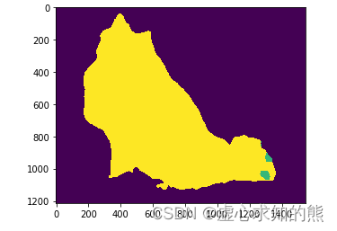
我们可以使用 hub 模块中的模型绘制每种颜色 21 个类别的语义分割预测。

# plot the semantic segmentation predictions of 21 classes in each color
r = Image.fromarray(output_predictions.byte().cpu().numpy()).resize(input_image.size)
r.putpalette(colors)

import matplotlib.pyplot as plt
plt.imshow(r)
plt.show()

在这里插入图片描述

二、搭建神经网络进行气温预测

1. 数据信息处理

在最开始，我们需要导入必备的库。

import numpy as np
import pandas as pd 
import matplotlib.pyplot as plt
import torch
import torch.optim as optim
import warnings
warnings.filterwarnings("ignore")%matplotlib inline

我们需要观察一下自己的数据都有哪些信息，在此之前，我们需要进行数据的读入，并打印数据的前五行进行观察。

features = pd.read_csv('temps.csv')
features.head()#year    month    day    week    temp_2    temp_1    average    actual    friend#0    2016    1    1    Fri    45    45    45.6    45    29#1    2016    1    2    Sat    44    45    45.7    44    61#2    2016    1    3    Sun    45    44    45.8    41    56#3    2016    1    4    Mon    44    41    45.9    40    53#4    2016    1    5    Tues    41    40    46.0    44    41

在我们的数据表中，包含如下数据信息：
（1） year 表示年数时间信息。
（2） month 表示月数时间信息。
（3） day 表示天数时间信息。
（4） week 表示周数时间信息。
（5） temp_2 表示前天的最高温度值。
（6） temp_1 表示昨天的最高温度值。
（7） average 表示在历史中，每年这一天的平均最高温度值。
（8） actual 表示这就是我们的标签值了，当天的真实最高温度。
（9） friend 表示这一列可能是凑热闹的，你的朋友猜测的可能值，咱们不管它就好了。
在获悉每一个数据的信息之后，我们需要知道一共有多少个数据。

print('数据维度:', features.shape)#数据维度: (348, 9)

(348, 9) 表示一共有 348 天，每一天有 9 个数据特征。
对于这么多的数据，直接进行行和列的操作可能会不太容易，因此，我们可以导入时间数据模块，将其转换为标准的时间信息。

# 处理时间数据import datetime

# 分别得到年，月，日
years = features['year']
months = features['month']
days = features['day']

# datetime格式
dates =[str(int(year))+'-'+str(int(month))+'-'+str(int(day))for year, month, day inzip(years, months, days)]
dates =[datetime.datetime.strptime(date,'%Y-%m-%d')for date in dates]

我们可以读取新列 dates 中的部分数据。

dates[:5]#[datetime.datetime(2016, 1, 1, 0, 0),# datetime.datetime(2016, 1, 2, 0, 0),# datetime.datetime(2016, 1, 3, 0, 0),# datetime.datetime(2016, 1, 4, 0, 0),# datetime.datetime(2016, 1, 5, 0, 0)]

2. 数据图画绘制

在基本数据处理完成后，我们就开始图画的绘制，在最开始，需要指定为默认的风格。

plt.style.use('fivethirtyeight')

设置布局信息。

# 设置布局
fig,((ax1, ax2),(ax3, ax4))= plt.subplots(nrows=2, ncols=2, figsize =(10,10))
fig.autofmt_xdate(rotation =45)

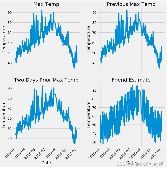
设置标签值信息。

#标签值
ax1.plot(dates, features['actual'])
ax1.set_xlabel(''); ax1.set_ylabel('Temperature'); ax1.set_title('Max Temp')

绘制昨天也就是 temp_1 的数据图画。

# 昨天
ax2.plot(dates, features['temp_1'])
ax2.set_xlabel(''); ax2.set_ylabel('Temperature'); ax2.set_title('Previous Max Temp')

绘制前天也就是 temp_2 的数据图画。

# 前天
ax3.plot(dates, features['temp_2'])
ax3.set_xlabel('Date'); ax3.set_ylabel('Temperature'); ax3.set_title('Two Days Prior Max Temp')

绘制朋友也就是 friend 的数据图画。

# 我的逗逼朋友
ax4.plot(dates, features['friend'])
ax4.set_xlabel('Date'); ax4.set_ylabel('Temperature'); ax4.set_title('Friend Estimate')

在上述信息设置完成后，开始图画的绘制。

plt.tight_layout(pad=2)

在这里插入图片描述

对原始数据中的信息进行编码，这里主要是指周数信息。

# 独热编码
features = pd.get_dummies(features)
features.head(5)#year    month    day    temp_2    temp_1    average    actual    friend    week_Fri    week_Mon    week_Sat    week_Sun    week_Thurs    week_Tues    week_Wed#0    2016    1    1    45    45    45.6    45    29    1    0    0    0    0    0    0#1    2016    1    2    44    45    45.7    44    61    0    0    1    0    0    0    0#2    2016    1    3    45    44    45.8    41    56    0    0    0    1    0    0    0#3    2016    1    4    44    41    45.9    40    53    0    1    0    0    0    0    0#4    2016    1    5    41    40    46.0    44    41    0    0    0    0    0    1    0

在周数信息编码完成后，我们将准确值进行标签操作，在特征数据中去掉标签数据，并将此时数据特征中的标签信息保存一下，并将其转换成合适的格式。

# 标签
labels = np.array(features['actual'])

# 在特征中去掉标签
features= features.drop('actual', axis =1)

# 名字单独保存一下，以备后患
feature_list =list(features.columns)

# 转换成合适的格式
features = np.array(features)

我们可以查看此时特征数据的具体数量。

features.shape
#(348, 14)

(348, 14) 表示我们的特征数据当中一共有 348 个，每一个有 14 个特征。
我们可以查看第一个的具体数据。

from sklearn import preprocessing
input_features = preprocessing.StandardScaler().fit_transform(features)
input_features[0]#array([ 0.        , -1.5678393 , -1.65682171, -1.48452388, -1.49443549,#       -1.3470703 , -1.98891668,  2.44131112, -0.40482045, -0.40961596,#       -0.40482045, -0.40482045, -0.41913682, -0.40482045])

3. 构建网络模型

x = torch.tensor(input_features, dtype =float)

y = torch.tensor(labels, dtype =float)

# 权重参数初始化
weights = torch.randn((14,128), dtype =float, requires_grad =True) 
biases = torch.randn(128, dtype =float, requires_grad =True) 
weights2 = torch.randn((128,1), dtype =float, requires_grad =True) 
biases2 = torch.randn(1, dtype =float, requires_grad =True) 

learning_rate =0.001 
losses =[]

for i inrange(1000):# 计算隐层
    hidden = x.mm(weights)+ biases
    # 加入激活函数
    hidden = torch.relu(hidden)# 预测结果
    predictions = hidden.mm(weights2)+ biases2
    # 通计算损失
    loss = torch.mean((predictions - y)**2) 
    losses.append(loss.data.numpy())# 打印损失值if i %100==0:print('loss:', loss)#返向传播计算
    loss.backward()#更新参数
    weights.data.add_(- learning_rate * weights.grad.data)  
    biases.data.add_(- learning_rate * biases.grad.data)
    weights2.data.add_(- learning_rate * weights2.grad.data)
    biases2.data.add_(- learning_rate * biases2.grad.data)# 每次迭代都得记得清空
    weights.grad.data.zero_()
    biases.grad.data.zero_()
    weights2.grad.data.zero_()
    biases2.grad.data.zero_()
#loss: tensor(8347.9924, dtype=torch.float64, grad_fn=<MeanBackward0>)#loss: tensor(152.3170, dtype=torch.float64, grad_fn=<MeanBackward0>)#loss: tensor(145.9625, dtype=torch.float64, grad_fn=<MeanBackward0>)#loss: tensor(143.9453, dtype=torch.float64, grad_fn=<MeanBackward0>)#loss: tensor(142.8161, dtype=torch.float64, grad_fn=<MeanBackward0>)#loss: tensor(142.0664, dtype=torch.float64, grad_fn=<MeanBackward0>)#loss: tensor(141.5386, dtype=torch.float64, grad_fn=<MeanBackward0>)#loss: tensor(141.1528, dtype=torch.float64, grad_fn=<MeanBackward0>)#loss: tensor(140.8618, dtype=torch.float64, grad_fn=<MeanBackward0>)#loss: tensor(140.6318, dtype=torch.float64, grad_fn=<MeanBackward0>)

我们查看预测数据的具体数量，应该是一共有 348 个，每个只有一个值，也就是 (348，1)。

predictions.shape
#torch.Size([348, 1])

4. 更简单的构建网络模型

input_size = input_features.shape[1]
hidden_size =128
output_size =1
batch_size =16
my_nn = torch.nn.Sequential(
    torch.nn.Linear(input_size, hidden_size),
    torch.nn.Sigmoid(),
    torch.nn.Linear(hidden_size, output_size),)
cost = torch.nn.MSELoss(reduction='mean')
optimizer = torch.optim.Adam(my_nn.parameters(), lr =0.001)# 训练网络
losses =[]for i inrange(1000):
    batch_loss =[]# MINI-Batch方法来进行训练for start inrange(0,len(input_features), batch_size):
        end = start + batch_size if start + batch_size <len(input_features)elselen(input_features)
        xx = torch.tensor(input_features[start:end], dtype = torch.float, requires_grad =True)
        yy = torch.tensor(labels[start:end], dtype = torch.float, requires_grad =True)
        prediction = my_nn(xx)
        loss = cost(prediction, yy)
        optimizer.zero_grad()
        loss.backward(retain_graph=True)
        optimizer.step()
        batch_loss.append(loss.data.numpy())# 打印损失if i %100==0:
        losses.append(np.mean(batch_loss))print(i, np.mean(batch_loss))#0 3950.7627#100 37.9201#200 35.654438#300 35.278366#400 35.116814#500 34.986076#600 34.868954#700 34.75414#800 34.637356#900 34.516705

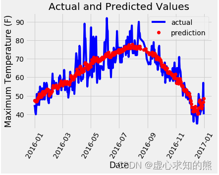
我们可以得到如下的预测训练结果，将其用图画的形式展现出来。

x = torch.tensor(input_features, dtype = torch.float)
predict = my_nn(x).data.numpy()# 转换日期格式
dates =[str(int(year))+'-'+str(int(month))+'-'+str(int(day))for year, month, day inzip(years, months, days)]
dates =[datetime.datetime.strptime(date,'%Y-%m-%d')for date in dates]

# 创建一个表格来存日期和其对应的标签数值
true_data = pd.DataFrame(data ={'date': dates,'actual': labels})

# 同理，再创建一个来存日期和其对应的模型预测值
months = features[:, feature_list.index('month')]
days = features[:, feature_list.index('day')]
years = features[:, feature_list.index('year')]

test_dates =[str(int(year))+'-'+str(int(month))+'-'+str(int(day))for year, month, day inzip(years, months, days)]

test_dates =[datetime.datetime.strptime(date,'%Y-%m-%d')for date in test_dates]

predictions_data = pd.DataFrame(data ={'date': test_dates,'prediction': predict.reshape(-1)})# 真实值
plt.plot(true_data['date'], true_data['actual'],'b-', label ='actual')

# 预测值
plt.plot(predictions_data['date'], predictions_data['prediction'],'ro', label ='prediction')
plt.xticks(rotation ='60'); 
plt.legend()

# 图名
plt.xlabel('Date'); plt.ylabel('Maximum Temperature (F)'); plt.title('Actual and Predicted Values');

在这里插入图片描述

标签： pytorch 神经网络人工智能

本文转载自: https://blog.csdn.net/weixin_45891612/article/details/129625581
版权归原作者 虚心求知的熊 所有，如有侵权，请联系我们删除。

PyTorch 之强大的 hub 模块和搭建神经网络进行气温预测

文章目录

一、强大的 hub 模块

1. hub 模块的使用

2. hub 模块的代码演示

二、搭建神经网络进行气温预测

1. 数据信息处理

2. 数据图画绘制

3. 构建网络模型

4. 更简单的构建网络模型

发表评论

“PyTorch 之强大的 hub 模块和搭建神经网络进行气温预测”的评论:

关于作者

overfit同步小助手

相关阅读

文章导航

PyTorch 之 强大的 hub 模块和搭建神经网络进行气温预测

文章目录

一、强大的 hub 模块

1. hub 模块的使用

2. hub 模块的代码演示

二、搭建神经网络进行气温预测

1. 数据信息处理

2. 数据图画绘制

3. 构建网络模型

4. 更简单的构建网络模型

发表评论

“PyTorch 之 强大的 hub 模块和搭建神经网络进行气温预测”的评论:

关于作者

overfit同步小助手

相关阅读

文章导航

PyTorch 之强大的 hub 模块和搭建神经网络进行气温预测

“PyTorch 之强大的 hub 模块和搭建神经网络进行气温预测”的评论: