
1.二维绘图
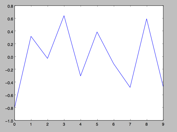
a. 一维数据集
用 Numpy ndarray 作为数据传入 ply
import numpy as np
import matplotlib as mpl
import matplotlib.pyplot as plt

np.random.seed(1000)
y = np.random.standard_normal(10)
print "y = %s"% y
x = range(len(y))
print "x=%s"% x
plt.plot(y)
plt.show()

2.操纵坐标轴和增加网格及标签的函数
import numpy as np
import matplotlib as mpl
import matplotlib.pyplot as plt

np.random.seed(1000)
y = np.random.standard_normal(10)
plt.plot(y.cumsum())
plt.grid(True) ##增加格点
plt.axis('tight') # 坐标轴适应数据量 axis 设置坐标轴
plt.show()

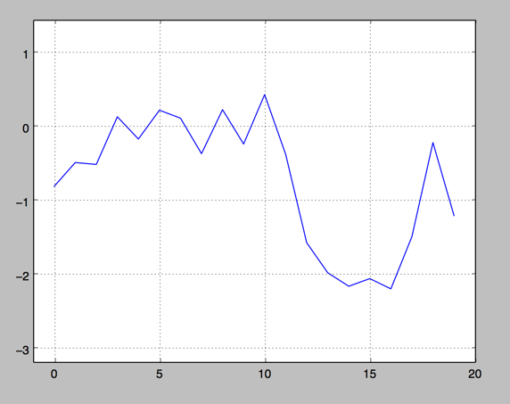
3.plt.xlim 和 plt.ylim 设置每个坐标轴的最小值和最大值
#!/etc/bin/python
#coding=utf-8
import numpy as np
import matplotlib as mpl
import matplotlib.pyplot as plt

np.random.seed(1000)
y = np.random.standard_normal(20)
plt.plot(y.cumsum())
plt.grid(True) ##增加格点
plt.xlim(-1,20)
plt.ylim(np.min(y.cumsum())- 1, np.max(y.cumsum()) + 1)

plt.show()
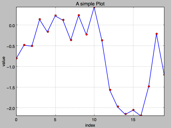
- 添加标题和标签 plt.title, plt.xlabe, plt.ylabel 离散点, 线
#!/etc/bin/python
#coding=utf-8
import numpy as np
import matplotlib as mpl
import matplotlib.pyplot as plt

np.random.seed(1000)
y = np.random.standard_normal(20)

plt.figure(figsize=(7,4)) #画布大小
plt.plot(y.cumsum(),'b',lw = 1.5) # 蓝色的线
plt.plot(y.cumsum(),'ro') #离散的点
plt.grid(True)
plt.axis('tight')
plt.xlabel('index')
plt.ylabel('value')
plt.title('A simple Plot')
plt.show()
b. 二维数据集
np.random.seed(2000)
y = np.random.standard_normal((10, 2)).cumsum(axis=0)   #10行2列   在这个数组上调用cumsum 计算赝本数据在0轴(即第一维)上的总和
print y

1.两个数据集绘图
#!/etc/bin/python
#coding=utf-8
import numpy as np
import matplotlib as mpl
import matplotlib.pyplot as plt

np.random.seed(2000)
y = np.random.standard_normal((10, 2))
plt.figure(figsize=(7,5))
plt.plot(y, lw = 1.5)
plt.plot(y, 'ro')
plt.grid(True)
plt.axis('tight')
plt.xlabel('index')
plt.ylabel('value')
plt.title('A simple plot')
plt.show()

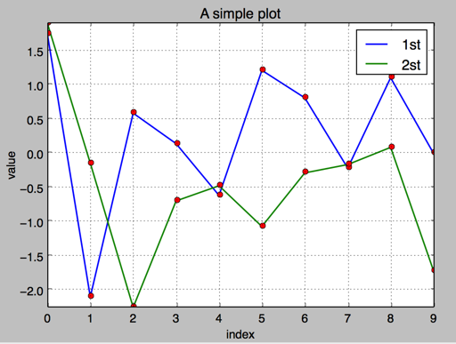
2.添加图例 plt.legend(loc = 0)
#!/etc/bin/python
#coding=utf-8
import numpy as np
import matplotlib as mpl
import matplotlib.pyplot as plt

np.random.seed(2000)
y = np.random.standard_normal((10, 2))
plt.figure(figsize=(7,5))
plt.plot(y[:,0], lw = 1.5,label = '1st')
plt.plot(y[:,1], lw = 1.5, label = '2st')
plt.plot(y, 'ro')
plt.grid(True)
plt.legend(loc = 0) #图例位置自动
plt.axis('tight')
plt.xlabel('index')
plt.ylabel('value')
plt.title('A simple plot')
plt.show()
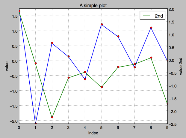
3.使用2个 Y轴(左右)fig, ax1 = plt.subplots() ax2 = ax1.twinx()
#!/etc/bin/python
#coding=utf-8
import numpy as np
import matplotlib as mpl
import matplotlib.pyplot as plt

np.random.seed(2000)
y = np.random.standard_normal((10, 2))

fig, ax1 = plt.subplots() # 关键代码1 plt first data set using first (left) axis

plt.plot(y[:,0], lw = 1.5,label = '1st')

plt.plot(y[:,0], 'ro')
plt.grid(True)
plt.legend(loc = 0) #图例位置自动
plt.axis('tight')
plt.xlabel('index')
plt.ylabel('value')
plt.title('A simple plot')

ax2 = ax1.twinx()  #关键代码2  plt second data set using second(right) axis
plt.plot(y[:,1],'g', lw = 1.5, label = '2nd')
plt.plot(y[:,1], 'ro')
plt.legend(loc = 0)
plt.ylabel('value 2nd')
plt.show()
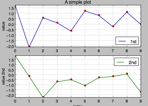
4.使用两个子图(上下,左右)plt.subplot(211)
通过使用 plt.subplots 函数,可以直接访问底层绘图对象,例如可以用它生成和第一个子图共享 x 轴的第二个子图.
#!/etc/bin/python
#coding=utf-8
import numpy as np
import matplotlib as mpl
import matplotlib.pyplot as plt

np.random.seed(2000)
y = np.random.standard_normal((10, 2))

plt.figure(figsize=(7,5))
plt.subplot(211)  #两行一列,第一个图
plt.plot(y[:,0], lw = 1.5,label = '1st')
plt.plot(y[:,0], 'ro')
plt.grid(True)
plt.legend(loc = 0) #图例位置自动
plt.axis('tight')
plt.ylabel('value')
plt.title('A simple plot')

plt.subplot(212) #两行一列.第二个图
plt.plot(y[:,1],'g', lw = 1.5, label = '2nd')
plt.plot(y[:,1], 'ro')
plt.grid(True)
plt.legend(loc = 0)
plt.xlabel('index')
plt.ylabel('value 2nd')
plt.axis('tight')
plt.show()
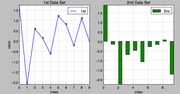
5.左右子图
有时候,选择两个不同的图标类型来可视化数据可能是必要的或者是理想的.利用子图方法:
#!/etc/bin/python
#coding=utf-8
import numpy as np
import matplotlib as mpl
import matplotlib.pyplot as plt

np.random.seed(2000)
y = np.random.standard_normal((10, 2))

plt.figure(figsize=(10,5))
plt.subplot(121)  #两行一列,第一个图
plt.plot(y[:,0], lw = 1.5,label = '1st')
plt.plot(y[:,0], 'ro')
plt.grid(True)
plt.legend(loc = 0) #图例位置自动
plt.axis('tight')
plt.xlabel('index')
plt.ylabel('value')
plt.title('1st Data Set')

plt.subplot(122)
plt.bar(np.arange(len(y)), y[:,1],width=0.5, color='g',label = '2nc')
plt.grid(True)
plt.legend(loc=0)
plt.axis('tight')
plt.xlabel('index')
plt.title('2nd Data Set')
plt.show()
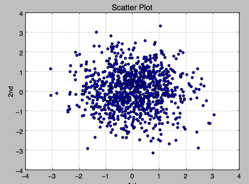
c.其他绘图样式,散点图,直方图等
1.散点图 scatter
#!/etc/bin/python
#coding=utf-8
import numpy as np
import matplotlib as mpl
import matplotlib.pyplot as plt

np.random.seed(2000)
y = np.random.standard_normal((1000, 2))
plt.figure(figsize=(7,5))
plt.scatter(y[:,0],y[:,1],marker='o')
plt.grid(True)
plt.xlabel('1st')
plt.ylabel('2nd')
plt.title('Scatter Plot')
plt.show()
2.直方图 plt.hist
#!/etc/bin/python
#coding=utf-8
import numpy as np
import matplotlib as mpl
import matplotlib.pyplot as plt

np.random.seed(2000)
y = np.random.standard_normal((1000, 2))
plt.figure(figsize=(7,5))
plt.hist(y,label=['1st','2nd'],bins=25)
plt.grid(True)
plt.xlabel('value')
plt.ylabel('frequency')
plt.title('Histogram')
plt.show()

3.直方图 同一个图中堆叠
#!/etc/bin/python
#coding=utf-8
import numpy as np
import matplotlib as mpl
import matplotlib.pyplot as plt

np.random.seed(2000)
y = np.random.standard_normal((1000, 2))
plt.figure(figsize=(7,5))
plt.hist(y,label=['1st','2nd'],color=['b','g'],stacked=True,bins=20)
plt.grid(True)
plt.xlabel('value')
plt.ylabel('frequency')
plt.title('Histogram')
plt.show()

4.箱型图 boxplot
#!/etc/bin/python
#coding=utf-8
import numpy as np
import matplotlib as mpl
import matplotlib.pyplot as plt

np.random.seed(2000)
y = np.random.standard_normal((1000, 2))
fig, ax = plt.subplots(figsize=(7,4))
plt.boxplot(y)

plt.grid(True)
plt.setp(ax,xticklabels=['1st' , '2nd'])
plt.xlabel('value')
plt.ylabel('frequency')
plt.title('Histogram')
plt.show()

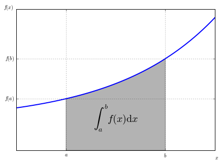
5.绘制函数
from matplotlib.patches import Polygon
import numpy as np
import matplotlib.pyplot as plt

#1. 定义积分函数
def func(x):
    return 0.5 * np.exp(x)+1

#2.定义积分区间
a,b = 0.5, 1.5
x = np.linspace(0, 2 )
y = func(x)
#3.绘制函数图形
fig, ax = plt.subplots(figsize=(7,5))
plt.plot(x,y, 'b',linewidth=2)
plt.ylim(ymin=0)
#4.核心, 我们使用Polygon函数生成阴影部分,表示积分面积:
Ix = np.linspace(a,b)
Iy = func(Ix)
verts = [(a,0)] + list(zip(Ix, Iy))+[(b,0)]
poly = Polygon(verts,facecolor='0.7',edgecolor = '0.5')
ax.add_patch(poly)
#5.用plt.text和plt.figtext在图表上添加数学公式和一些坐标轴标签。
plt.text(0.5 *(a+b),1,r"$\int_a^b f(x)\mathrm{d}x$", horizontalalignment ='center',fontsize=20)
plt.figtext(0.9, 0.075,'$x$')
plt.figtext(0.075, 0.9, '$f(x)$')
#6. 分别设置x,y刻度标签的位置。
ax.set_xticks((a,b))
ax.set_xticklabels(('$a$','$b$'))
ax.set_yticks([func(a),func(b)])
ax.set_yticklabels(('$f(a)$','$f(b)$'))
plt.grid(True)
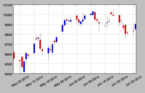
2.金融学图表 matplotlib.finance
1.烛柱图 candlestick
#!/etc/bin/python
#coding=utf-8
import matplotlib.pyplot as plt
import matplotlib.finance as mpf
start = (2014, 5,1)
end = (2014, 7,1)
quotes = mpf.quotes_historical_yahoo('^GDAXI',start,end)
# print quotes[:2]

fig, ax = plt.subplots(figsize=(8,5))
fig.subplots_adjust(bottom = 0.2)
mpf.candlestick(ax, quotes, width=0.6, colorup='b',colordown='r')
plt.grid(True)
ax.xaxis_date() #x轴上的日期
ax.autoscale_view()
plt.setp(plt.gca().get_xticklabels(),rotation=30) #日期倾斜
plt.show()
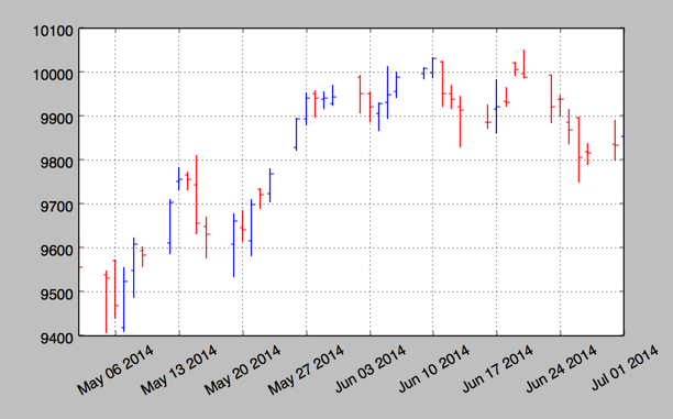
- plot_day_summary
该函数提供了一个相当类似的图标类型,使用方法和 candlestick 函数相同,使用类似的参数. 这里开盘价和收盘价不是由彩色矩形表示,而是由两条短水平线表示.
#!/etc/bin/python
#coding=utf-8
import matplotlib.pyplot as plt
import matplotlib.finance as mpf
start = (2014, 5,1)
end = (2014, 7,1)
quotes = mpf.quotes_historical_yahoo('^GDAXI',start,end)
# print quotes[:2]

fig, ax = plt.subplots(figsize=(8,5))
fig.subplots_adjust(bottom = 0.2)
mpf.plot_day_summary(ax, quotes,  colorup='b',colordown='r')
plt.grid(True)
ax.xaxis_date() #x轴上的日期
ax.autoscale_view()
plt.setp(plt.gca().get_xticklabels(),rotation=30) #日期倾斜
plt.show()
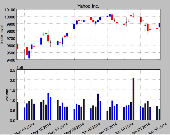
3.股价数据和成交量
#!/etc/bin/python
#coding=utf-8
import matplotlib.pyplot as plt
import numpy as np
import matplotlib.finance as mpf
start = (2014, 5,1)
end = (2014, 7,1)
quotes = mpf.quotes_historical_yahoo('^GDAXI',start,end)
# print quotes[:2]

quotes = np.array(quotes)
fig, (ax1, ax2) = plt.subplots(2, sharex=True, figsize=(8,6))
mpf.candlestick(ax1, quotes, width=0.6,colorup='b',colordown='r')
ax1.set_title('Yahoo Inc.')
ax1.set_ylabel('index level')
ax1.grid(True)
ax1.xaxis_date()
plt.bar(quotes[:,0] - 0.25, quotes[:, 5], width=0.5)

ax2.set_ylabel('volume')
ax2.grid(True)
ax2.autoscale_view()
plt.setp(plt.gca().get_xticklabels(),rotation=30)
plt.show()
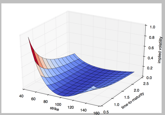
3.3D 绘图
#!/etc/bin/python
#coding=utf-8
import numpy as np
import matplotlib.pyplot as plt

stike = np.linspace(50, 150, 24)
ttm = np.linspace(0.5, 2.5, 24)
stike, ttm = np.meshgrid(stike, ttm)
print  stike[:2]

iv = (stike - 100) ** 2 / (100 * stike) /ttm
from mpl_toolkits.mplot3d import Axes3D
fig = plt.figure(figsize=(9,6))
ax = fig.gca(projection='3d')
surf = ax.plot_surface(stike, ttm, iv, rstride=2, cstride=2, cmap=plt.cm.coolwarm, linewidth=0.5, antialiased=True)
ax.set_xlabel('strike')
ax.set_ylabel('time-to-maturity')
ax.set_zlabel('implied volatility')

plt.show()
岁
本文转载自: https://blog.csdn.net/m0_59485658/article/details/129371433
版权归原作者 代码输入中... 所有, 如有侵权,请联系我们删除。
版权归原作者 代码输入中... 所有, 如有侵权,请联系我们删除。