
在学习贝叶斯计算的解马尔可夫链蒙特卡洛(MCMC)模拟时,最简单的方法是使用PyMC3,构建模型,调用Metropolis优化器。但是使用别人的包我们并不真正理解发生了什么,所以本文通过手写Metropolis-Hastings来深入的理解MCMC的过程,再次强调我们自己实现该方法并不是并不是为了造轮子,而是为了更好的通过代码理解该概念。
贝叶斯线性回归包含了几十个概念和定义,这使得我们的整个研究成为一种折磨,并且真正发生的事情。在本文中,我将通过常见Metropolis-Hastings 算法构建一个马尔可夫链,并提供一个实际的使用案例。我们将着重于推断简单线性回归模型的参数(但是这里说“简单”并不能代表它背后的原理简单)。我们还可以用任何其他条件分布(泊松/伽马/负二项或其他)替换正态分布,这样可以通过MCMC实现几乎相同的GLM(只更改4或5行代码)。由于推断的样本来自参数的后验分布,我们可以很自然地使用这些来构建参数的置信区间(在这种情况下,“可信区间”更正确)。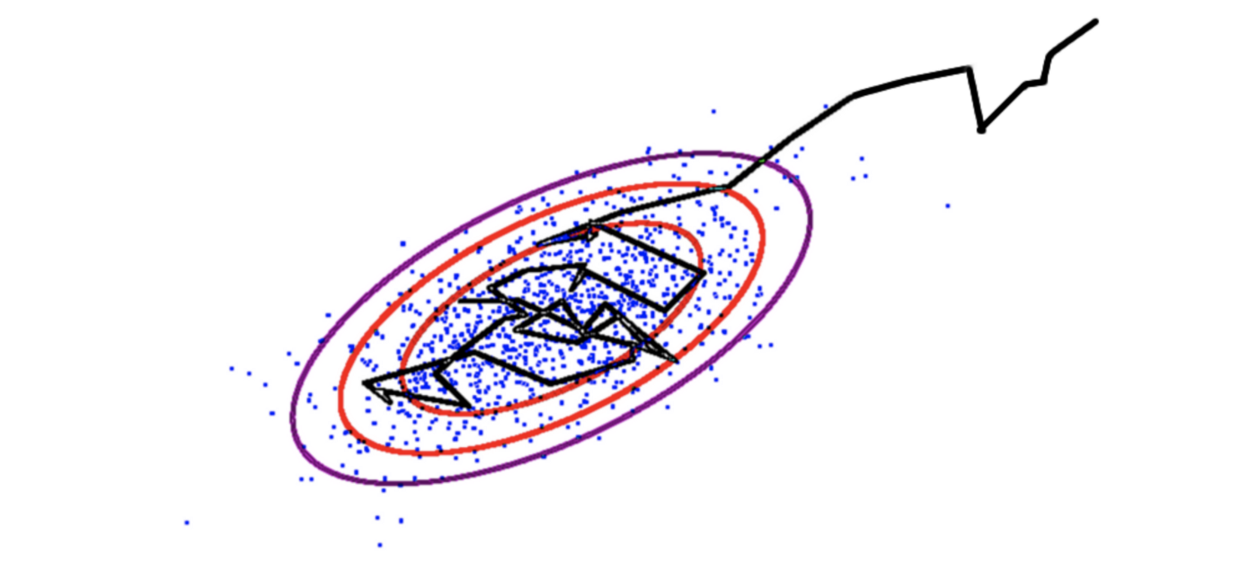
下面我们将简要描述为什么使用MCMC方法,提供一个线性回归模型的MH算法的实现,并将以一个可视化的方式显示当算法寻找生成数据的参数集时,真正发生了什么。
数据准备
设Y和X分别为模型的响应和输入。线性模型表明,给定输入的响应的条件分布是正态的。也就是:
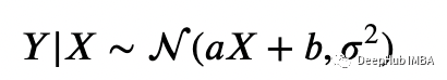
对于合适的参数a(斜率)、b(偏差)和σ(噪声强度)。
我们的任务是推断a, b和σ。
所以我们首先要知道一些模型需要遵循的“基本规则”。在这个例子中,a, b几乎可以是任何数值,正的或负的,但σ必须是严格正的(因为从来没有听说过负标准差的正态分布,对吧?)除此之外,没有其他任何规则。也许你会说:“我们需要先了解这些是如何分布的”,但是后验分布的渐近正态性保证告诉我们,只要有足够的后验样本,这些样本无论如何都是正态分布(如果马尔可夫链达到其平稳分布),所以分布不是我们考虑的必要因素。
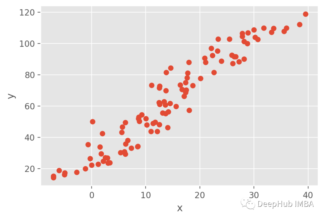
现在让我们为回归生成合成数据,这里使用参数a=3, b=20和σ=5。可以通过以下代码在python中完成:
import numpy as np
import matplotlib.pyplot as plt
import scipy.stats as sc

# sample x
np.random.seed(2022)
x = np.random.rand(100)*30

# set parameters
a = 3
b = 20
sigma = 5

# obtain response and add noise
y = a*x+b
noise = np.random.randn(100)*sigma

# create a matrix containing the predictor in the first column
# and the response in the second
data = np.vstack((x,y)).T + noise.reshape(-1,1)

# plot data
plt.scatter(data[:,0], data[:,1])
plt.xlabel("x")
plt.ylabel("y")
合成数据如下图所示:
数据的准备已经完成了,下一节将涉及定义 Metropolis Hastings 算法的函数和一组迭代次数的循环。
算法介绍
假设θ=[a,b,σ]是算法上面的参数向量,θ '是一组新参数的建议,MH比较参数(θ '和θ)的两个竞争假设之间的贝叶斯因子(似然和先验的乘积),并通过条件建议分布的倒数缩放该因子。然后将该因子与均匀分布的随机变量的值进行比较。这给模型增加了随机性,使不可能的参数向量有可能被探索,也可能被丢弃(很少)。
这听起来有点复杂,让我们从头一步一步对它进行代码的实现。
Proposal Distribution
首先,我们定义了一个建议的分布(Proposal Distribution)g(θ′|θ):这是前一个时间步固定参数的分布。在我们的例子中,a和b可以是正的也可以是负的,因此一个自然的选择就是从一个以前一个迭代步骤为中心的多元正态分布中采样它们。我们可以从伽马分布中取样σ,这些分布的定义我们可以根据实际情况进行选择,但是一个更好的方法(这里我们将不涉及)是从逆伽马分布抽样σ。
因此,我们可以按照以下方式定义进行Proposal Distribution:
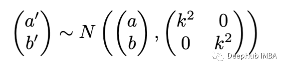
分布抽样σ为
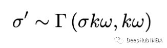
参数 k 用于控制分布在其均值周围的“扩展”。𝜔 是对gamma 额外调整。k𝜔越大,gamma 的分布越大(我们使用的是 gamma 分布的形状速率公式因为 scipy 强迫使用形状比例公式)。功能如下:
def proposal(prec_theta, search_width = 0.5):
    # this function generates the proposal for the new theta
    # we assume that the distribution of the random variables
    # is normal for the first two and gamma for the third.
    # conditional on the previous value of the accepted parameters (prec_theta)
    out_theta = np.zeros(3)
    out_theta[:2] = sc.multivariate_normal(mean=prec_theta[:2],cov=np.eye(2)*search_width**2).rvs(1)
    #the last component is the noise
    out_theta[2] = sc.gamma(a=prec_theta[2]*search_width*500, scale=1/(500*search_width)).rvs()
    return out_theta
我们可能会可以注意到函数proposal包含两个参数:prec_theta表示上面说的的参数向量,search_width表示寻找建议的区域。寻找一组良好的参数会在探索(在未探索的区域中搜索新参数集)和开发(在已找到良好参数集的区域中改进搜索)之间进行权衡。所以应该非常小心地设置search_width。search_width值过大会使MCMC收敛到平稳分布。一个小的值可能会阻止算法在合理的时间内找到最优(optima)(需要绘制更多的样本,更多的训练时间)。
似然函数
似然函数其实就是线性函数,并且给定参数的响应的条件分布是正态的。换句话说,我们将计算正态分布的可能性,其中均值是输入和系数a和b的乘积,噪声是σ。在这种情况下,我们将使用对数似然而不是原始似然,这样可以提高稳定性。
def lhd(x,theta):
    # x is the data matrix, first column for input and second column for output.
    # theta is a vector containing the parameters for the evaluation
    # remember theta[0] is a, theta[1] is b and theta[2] is sigma
    xs = x[:,0]
    ys = x[:,1]
    lhd_out = sc.norm.logpdf(ys, loc=theta[0]*xs+theta[1], scale=theta[2])
    # then we sum lhd_out (be careful here, we are summing instead of multiplying
    # because we are dealing with the log-likelihood, instead of the raw likelihood).
    lhd_out = np.sum(lhd_out)
    return lhd_out
先验
我们不需要在这方面花很多时间。在先验分布方面,可以选择任何喜欢的东西。这里需要做的就是确保可能找到推断的参数的区域具有非零先验,并且噪声参数 σ 是非负的。这里的先验以 log-pdf 的形式表示。
def prior(theta):
    # evaluate the prior for the parameters on a multivariate gaussian.
    prior_out = sc.multivariate_normal.logpdf(theta[:2],mean=np.array([0,0]), cov=np.eye(2)*100)
    # this needs to be summed to the prior for the sigma, since I assumed independence.
    prior_out += sc.gamma.logpdf(theta[2], a=1, scale=1)
    return prior_out
Proposal Ratio
Proposal Ratio是在给定新参数向量的情况下观察到旧参数向量的可能性除以给定旧参数向量的情况下观察到新参数向量的概率。也就是Proposal Distribution提到的,g(θ|θ′)/g(θ′|θ)。这里将使用log-pdf,这样可以在概率中具有统一的尺度,并获得更好的数值稳定性。
def proposal_ratio(theta_old, theta_new, search_width=10):
    # this is the proposal distribution ratio
    # first, we calculate of the pdf of the proposal distribution at the old value of theta with respect to the new
    # value of theta. And then we do the exact opposite.
    prop_ratio_out = sc.multivariate_normal.logpdf(theta_old[:2],mean=theta_new[:2], cov=np.eye(2)*search_width**2)
    prop_ratio_out += sc.gamma.logpdf(theta_old[2], a=theta_new[2]*walk*500, scale=1/(500*walk))
    prop_ratio_out -= sc.multivariate_normal.logpdf(theta_new[:2],mean=theta_old[:2], cov=np.eye(2)*search_width**2)
    prop_ratio_out -= sc.gamma.logpdf(theta_new[2], a=theta_old[2]*walk*500, scale=1/(500*walk))
    return prop_ratio_out
整合
把所有信息整合起来。伪代码如下:
1)实例化参数向量的初始值
... N次,直到收敛
2)从建议分布中找到一个新的参数向量
3)计算似然、先验pdf值和建议似然比的倒数
4)将3中的所有数量相乘(或log求和),并比较这个比例(线性比例)
根据从均匀分布中得出的数字。
5)如果比值较大,则接受新的参数向量。
否则,新的参数向量将被拒绝。
6)重复2
在Python代码如下:
np.random.seed(100)
width = 0.2

thetas = np.random.rand(3).reshape(1,-1)
accepted = 0
rejected = 0

N = 200000

for i in range(N):

    # 1) provide a proposal for theta
    theta_new = proposal(thetas[-1,:], search_width=width)

    # 2) calculate the likelihood of this proposal and the likelihood
    # for the old value of theta
    log_lik_theta_new = lhd(data,theta_new)
    log_lik_theta = lhd(data,thetas[-1,:])

    # 3) evaluate the prior log-pdf at the current and at the old value of theta
    theta_new_prior = prior(theta_new)
    theta_prior = prior(thetas[-1,:])

    # 4) finally, we need the proposal distribution ratio
    prop_ratio = proposal_ratio(thetas[-1], theta_new, search_width=width)

    # 5) assemble likelihood, priors and proposal distributions
    likelihood_prior_proposal_ratio = log_lik_theta_new - log_lik_theta + \
                             theta_new_prior - theta_prior + prop_ratio

    # 6) throw a - possibly infinitely weigthed - coin. The move for Metropolis-Hastings is
    # not deterministic. Here, we exponentiate the likelihood_prior_proposal ratio in order
    # to obtain the probability in linear scale
    if np.exp(likelihood_prior_proposal_ratio) > sc.uniform().rvs():
        thetas = np.vstack((thetas,theta_new))
        accepted += 1
    else:
        rejected += 1
上面的代码可能会要花费一些时间来运行。修改N来获得更少的采样,或编辑宽度以加快探索。
结果展示
结果包含在下图中
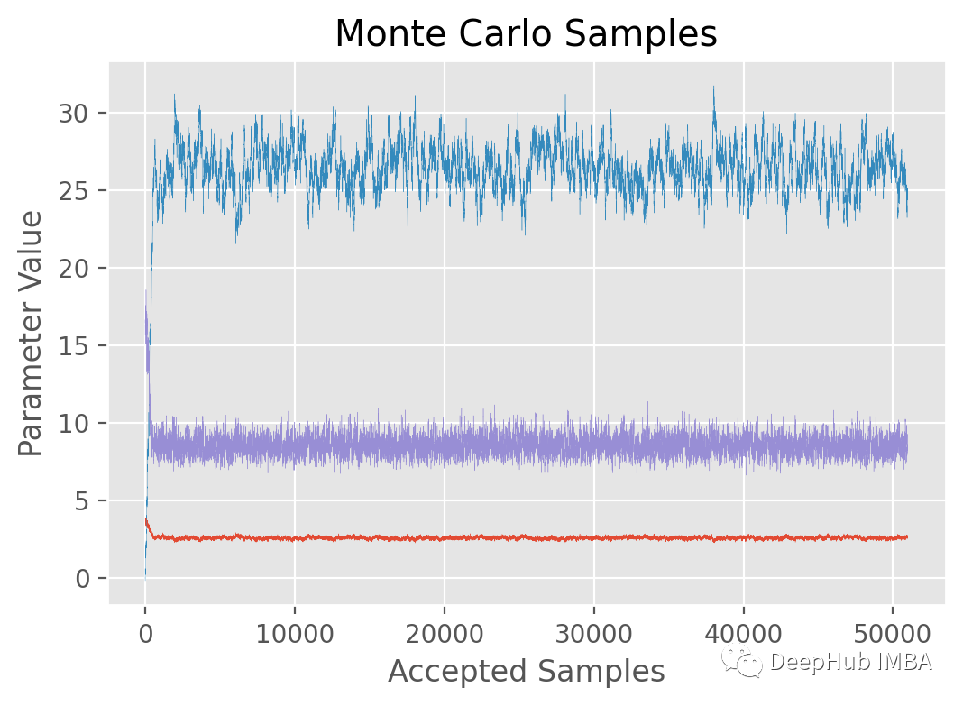
得到的:a(红色), b(蓝色) and σ(紫色)
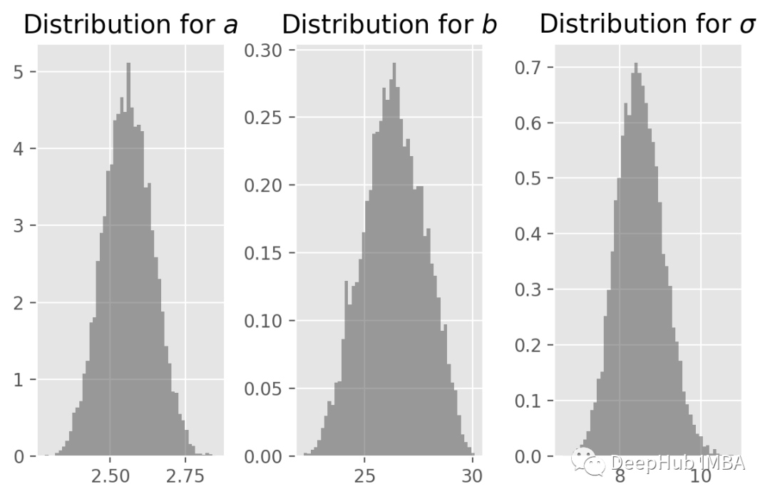
参数的直方图。
可以看到,样本的历史结果非常稳定。平均值和标准偏差是:
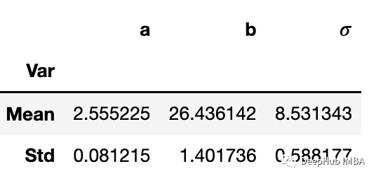
但是有一个问题,我们只在这里提一下:这些样本高度相关,因此在估计可信区间时可能需要小心。这里的一种解决方案是通过只保留一小部分参数来细化历史记录(例如,只保留1 / 10已接受的提议,并丢弃其余的)。
传统的线性回归相比如何呢?
使用 statsmodels.api.OLS 执行完全相同的计算
import statsmodels.api as sm
import pandas as pd

df = pd.DataFrame(data)
df.columns = ["a","y"]
df["b"] = 1
lm = sm.OLS(df["y"], df[["a","b"]]).fit()
lm.summary()
结果如下:
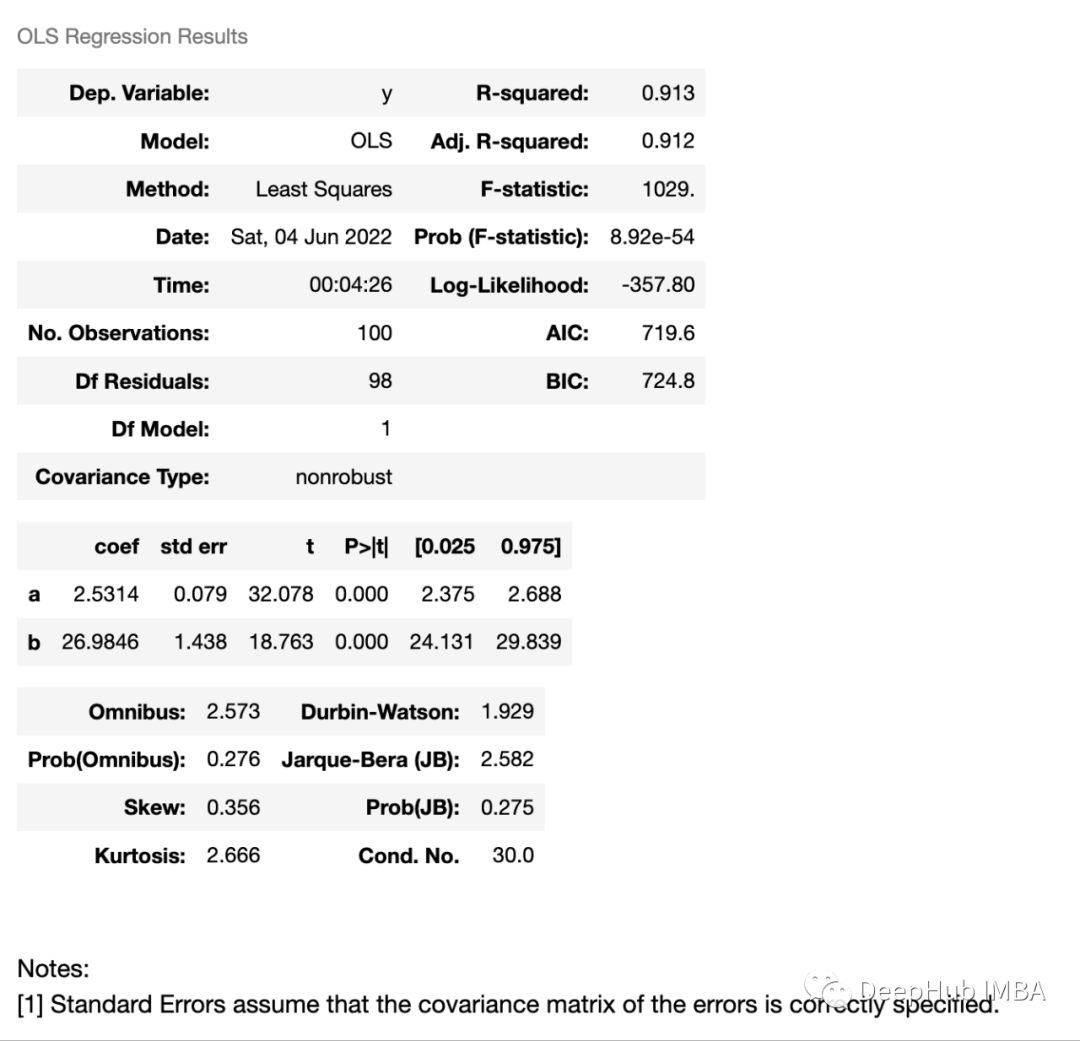
a 和 b 的系数的平均值非常接近 MCMC。标准误差也可以这样说,这样也进一步证明了我们对 MCMC 实现是可行的。
请注意,这不是最好的解决方案,而只是一个解决方案。因为确实存在并推荐更好的先验和建议分布的选择。
迭代的可视化?
在 3D 中可视化相当的混乱,所以这里只关注斜率 a 和偏差 b。
在可视化中,每 10 步显示一次 MH 的行为:
红点代表当前的建议提案,红点周围的灰色区域表示与平均值相差 3 个标准差的建议分布(正态)。该提案有一个对角协方差矩阵,这就是我们得到一个圆而不是椭圆。
蓝色线代表被拒绝的动作。
红线代表接受的动作
最上面浅蓝点表示从 statsmodels.api.OLS 获得的参数的平均值。
作者:Fortunato Nucera