
一、背景介绍
某通信公司是通信界的巨头,其用户流失率若降低5%,那么公司利润将提升25%-85%。如今随着市场饱和度上升,高居不下的获客成本让公司遭遇了“天花板”,甚至陷入获客难的窘境。增加用户黏性和延长用户生命周期成了该通信亟待解决的问题。
数据来源:https://www.kaggle.com/blastchar/telco-customer-churn
二、分析目的
1、分析流失用户特征,生成易流失用户标签;
2、预测用户留存率随时间的变化,并提出合理化召回建议。
三、分析思路

分析工具:Tableau、Mysql、python、excel
四、可视化分析用户流失
1、用户属性特征
用户的基本特征有:性别(Gender)、年龄(Senior,1:年长,2:年轻)、有无伴侣(Partner)、有无家属(Dependents),各特征用户的流失率如下图所示:
从图中看出,年长用户、有伴侣和有家属的用户流失率明显较高,用户性别对流失率的影响不大。
2、用户服务属性
用户服务属性有:电话服务(PhoneService)、多条线路(MultipleLines)、网络服务(InternetService)、网络安全服务(OnlineSecurity),各特征用户的流失率如下图所示:

从图中可以看出,网络服务为Fiber optic、没有网络安全服务的客户流失率最高,其次是网络服务为DSL、有网络安全服务的客户,没有网络服务和网络安全服务的用户流失率最低。
3、用户交易属性
用户交易属性有:合同期限(Contract)、付款方式(PaymentMethod)、每月付费金额(MonthlyCharges)、总付费金额(TotalCharges),各特征用户的流失率如下图所示:


从上图看出,合同期限为Month-to-month、付款方式为Electronic check、每月消费金额为70至100元、总消费300元以内的客户流失率最高。
4、小结
以下特征的用户最易流失:
1)年长用户、有伴侣、有家属;
2)网络服务为Fiber optic、没有网络安全服务;
3)同期限为Month-to-month、付款方式为Electronic check、每月消费金额为70至100元、总消费300元以内。
五、生成易流失等级标签
1、量化流失风险系数
各属性对用户流失的影响越大,则流失风险系数越高,具体划分如下: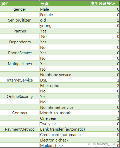
用Mysql取出未流失客户,并计算风险系数:
SELECT customerID,IF(SeniorCitizen=1,2,0)as senior,IF(Partner='Yes',2,0)as partner,IF(Dependents='Yes',2,0)as dependents,CASEWHEN InternetService='Fiber optic'THEN2WHEN InternetService='DSL'THEN1ELSE0ENDas internetservice,CASEWHEN OnlineSecurity='No'THEN2WHEN OnlineSecurity='Yes'THEN1ELSE0ENDas onlinesecurity,CASEWHEN Contract='Month-to-month'THEN2WHEN Contract='One year'THEN1ELSE0ENDas contract,CASEWHEN PaymentMethod='Electronic check'THEN2ELSE0ENDas paymentMethod,IF(MonthlyCharges>=70and MonthlyCharges <=100,1,0)as monthlycharges,IF(TotalCharges<300,1,0)as totalcharges
from ha.wa_fn;
查询结果如下: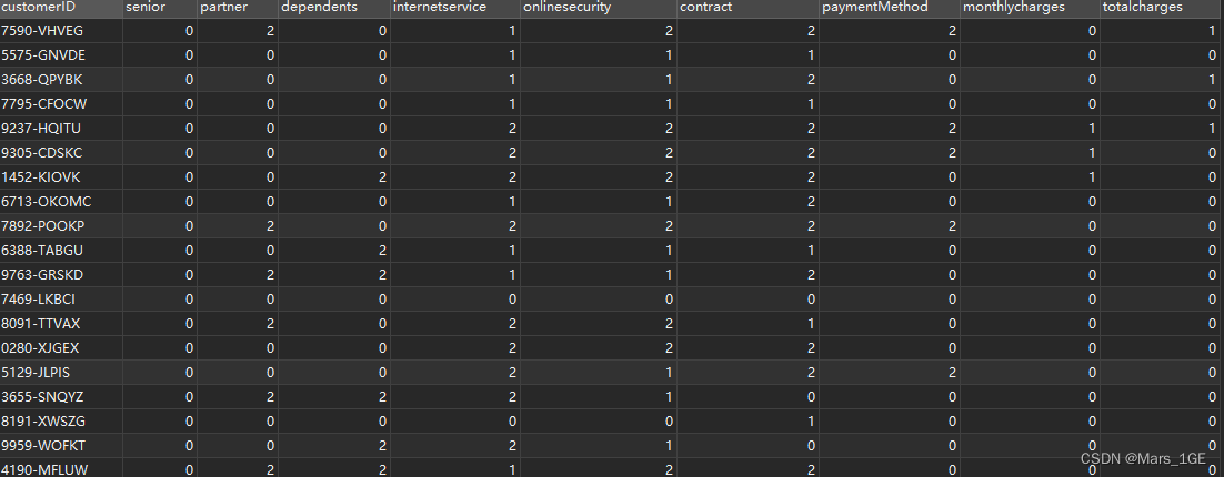
2、汇总风险系数,求出最终用户流失风险等级
将查询结果导入Excel中,求出最终的流失分析等级(churn_level):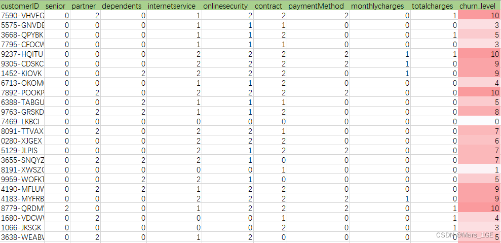
流失风险等级分布如下:
接下来,运营部同事就可以根据流失风险等级,分层运营客户。
3、添加高流失风险标签
比如,风险等级大于9的定义为高流失风险客户: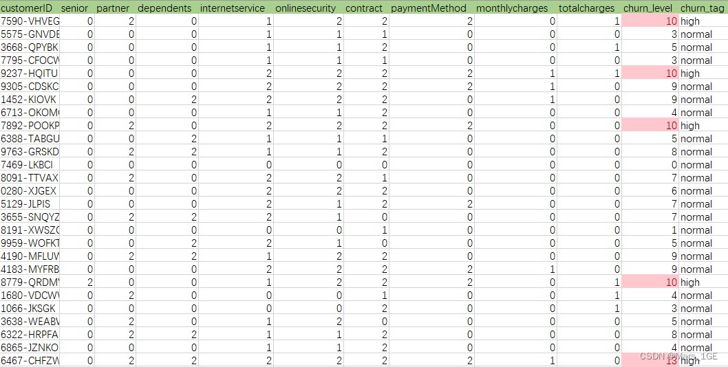
六、基于生存分析预测用户流失
1、导入模块
import pandas as pd
import numpy as np
import matplotlib.pyplot as plt
import seaborn as sns
from sklearn.preprocessing import LabelEncoder
from sklearn.model_selection import train_test_split
# 生存分析模块from lifelines import NelsonAalenFitter, CoxPHFitter, KaplanMeierFitter
from lifelines.statistics import logrank_test
# coxfrom lifelines import CoxPHFitter
from sklearn.metrics import brier_score_loss
from sklearn.calibration import calibration_curve
# matplotlib与pandas初始设置
plt.rcParams['font.sans-serif']=['SimHei']#设置中文字体为黑体
plt.rcParams['axes.unicode_minus']=False#正常显示负号
pd.set_option('display.max_columns',30)
plt.rcParams.update({"font.family":"SimHei","font.size":14})
plt.style.use("tableau-colorblind10")

pd.set_option('display.float_format',lambda x :'%.2f'% x)#pandas禁用科学计数法%matplotlib inline

#忽略警告import warnings
warnings.filterwarnings('ignore')
data = pd.read_csv('WA_Fn-UseC_-Telco-Customer-Churn.csv')
data_backup = data.copy()
data.head()
customerIDgenderSeniorCitizenPartnerDependentstenurePhoneServiceMultipleLinesInternetServiceOnlineSecurityOnlineBackupDeviceProtectionTechSupportStreamingTVStreamingMoviesContractPaperlessBillingPaymentMethodMonthlyChargesTotalChargesChurn07590-VHVEGFemale0YesNo1NoNo phone serviceDSLNoYesNoNoNoNoMonth-to-monthYesElectronic check29.8529.85No15575-GNVDEMale0NoNo34YesNoDSLYesNoYesNoNoNoOne yearNoMailed check56.951889.50No23668-QPYBKMale0NoNo2YesNoDSLYesYesNoNoNoNoMonth-to-monthYesMailed check53.85108.15Yes37795-CFOCWMale0NoNo45NoNo phone serviceDSLYesNoYesYesNoNoOne yearNoBank transfer (automatic)42.301840.75No49237-HQITUFemale0NoNo2YesNoFiber opticNoNoNoNoNoNoMonth-to-monthYesElectronic check70.70151.65Yes
2、数据预处理
# 缺失值
data.info()
<class 'pandas.core.frame.DataFrame'>
RangeIndex: 7043 entries, 0 to 7042
Data columns (total 21 columns):
 #   Column            Non-Null Count  Dtype
---  ------            --------------  -----
 0   customerID        7043 non-null   object
 1   gender            7043 non-null   object
 2   SeniorCitizen     7043 non-null   int64
 3   Partner           7043 non-null   object
 4   Dependents        7043 non-null   object
 5   tenure            7043 non-null   int64
 6   PhoneService      7043 non-null   object
 7   MultipleLines     7043 non-null   object
 8   InternetService   7043 non-null   object
 9   OnlineSecurity    7043 non-null   object
 10  OnlineBackup      7043 non-null   object
 11  DeviceProtection  7043 non-null   object
 12  TechSupport       7043 non-null   object
 13  StreamingTV       7043 non-null   object
 14  StreamingMovies   7043 non-null   object
 15  Contract          7043 non-null   object
 16  PaperlessBilling  7043 non-null   object
 17  PaymentMethod     7043 non-null   object
 18  MonthlyCharges    7043 non-null   float64
 19  TotalCharges      7043 non-null   object
 20  Churn             7043 non-null   object
dtypes: float64(1), int64(2), object(18)
memory usage: 1.1+ MB
# 由于TotalCharges列存在缺失值,所以强制转换成数字(info中并未显示缺失值,但如果正常转换就会报错)
data['TotalCharges']=pd.to_numeric(data['TotalCharges'],errors='coerce')
data['TotalCharges'].dtype
dtype('float64')
# 的确是存在缺失值
data.TotalCharges.isnull().sum()
11
# 删除缺失值
data.dropna(subset=['TotalCharges'],inplace=True)
# 重复值
data.duplicated('customerID').sum()
0
# 异常值
data.describe().T
countmeanstdmin25%50%75%maxSeniorCitizen7032.000.160.370.000.000.000.001.00tenure7032.0032.4224.551.009.0029.0055.0072.00MonthlyCharges7032.0064.8030.0918.2535.5970.3589.86118.75TotalCharges7032.002283.302266.7718.80401.451397.473794.748684.80
data.describe(include='object').T
countuniquetopfreqcustomerID703270327590-VHVEG1gender70322Male3549Partner70322No3639Dependents70322No4933PhoneService70322Yes6352MultipleLines70323No3385InternetService70323Fiber optic3096OnlineSecurity70323No3497OnlineBackup70323No3087DeviceProtection70323No3094TechSupport70323No3472StreamingTV70323No2809StreamingMovies70323No2781Contract70323Month-to-month3875PaperlessBilling70322Yes4168PaymentMethod70324Electronic check2365Churn70322No5163
3、分类数据转换
为了将数据代入模型,需要将分类数据转换成数字,这里用到了sklearn中的one-hoe-encode.
#分类数据转换为one-hoe-encode形式list=['gender','Partner','Dependents','PhoneService','MultipleLines','InternetService','OnlineSecurity','OnlineBackup','DeviceProtection','TechSupport','StreamingTV','StreamingMovies','Contract','PaperlessBilling','PaymentMethod','Churn']
lec = LabelEncoder()
data.loc[:,list]=data.loc[:,list].transform(lec.fit_transform)# churn:N0:0;Yes:1
data.head()
customerIDgenderSeniorCitizenPartnerDependentstenurePhoneServiceMultipleLinesInternetServiceOnlineSecurityOnlineBackupDeviceProtectionTechSupportStreamingTVStreamingMoviesContractPaperlessBillingPaymentMethodMonthlyChargesTotalChargesChurn07590-VHVEG0010101002000001229.8529.85015575-GNVDE10003410020200010356.951889.50023668-QPYBK1000210022000001353.85108.15137795-CFOCW10004501020220010042.301840.75049237-HQITU0000210100000001270.70151.651
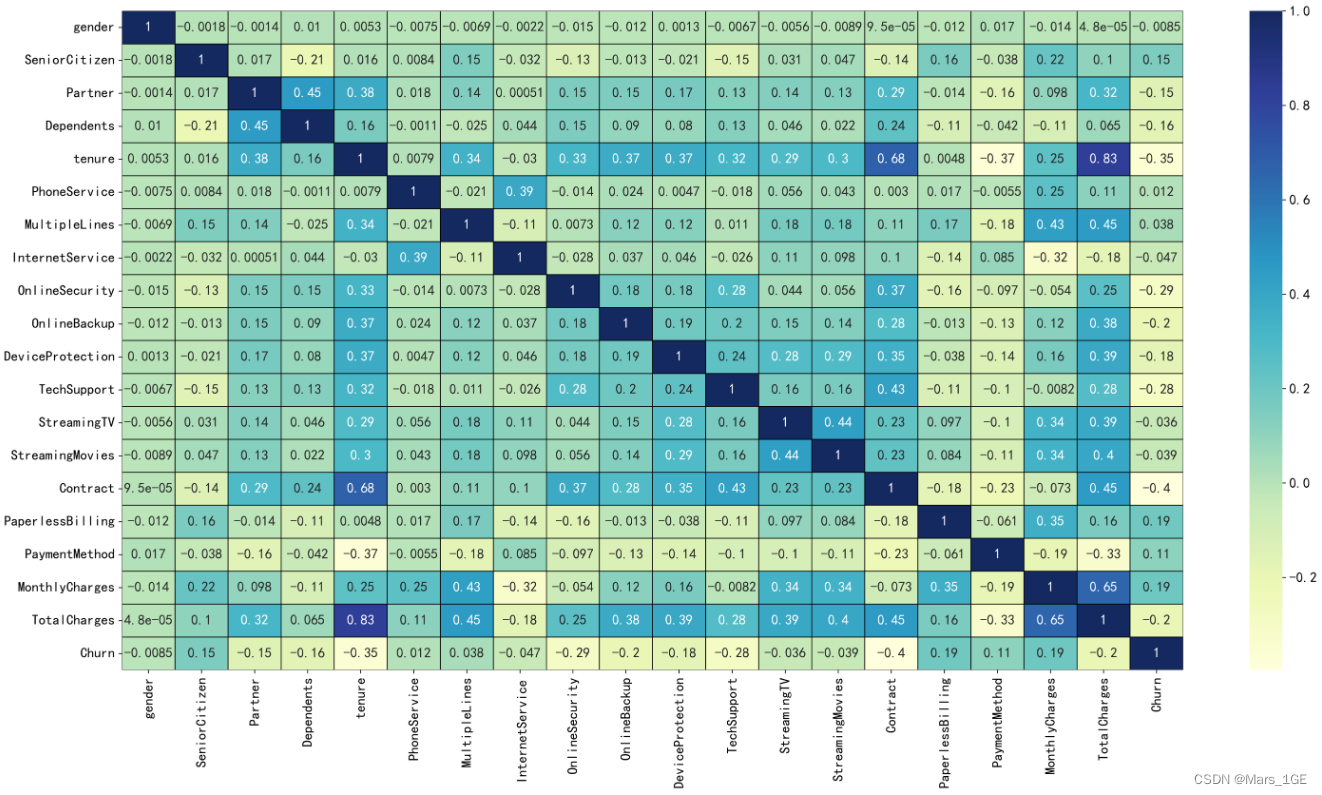
4、相关性分析
相关性热力图
fig = plt.figure(figsize=(24,12),dpi=600)
ax = sns.heatmap(data.corr(), cmap="YlGnBu",
      linecolor='black', lw=.65,annot=True, alpha=.95)
ax.set_xticklabels([x for x in data.drop('customerID',axis=1).columns])
ax.set_yticklabels([y for y in data.drop('customerID',axis=1).columns])
plt.show()
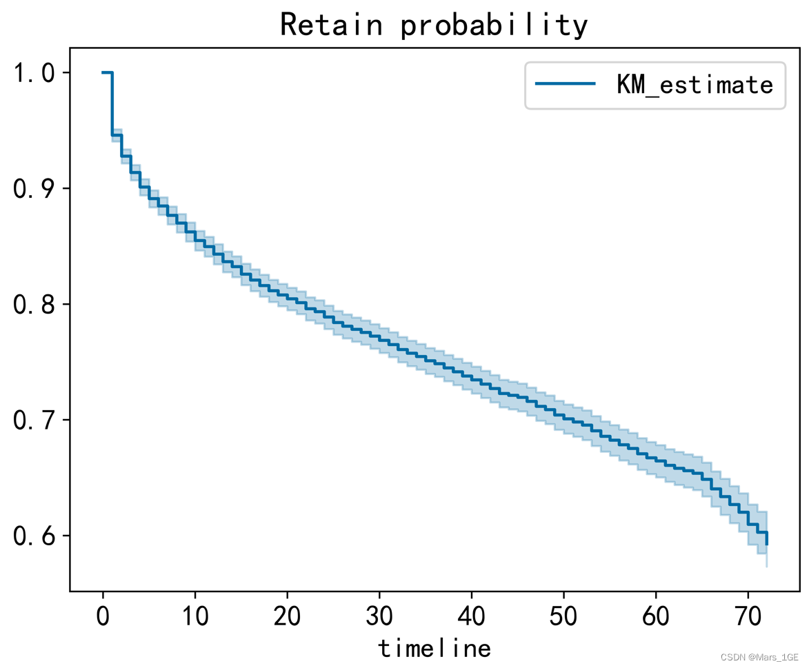
5、KM模型分析留存率
plt.figure(dpi=800)
kmf = KaplanMeierFitter()
kmf.fit(data['tenure'], event_observed=data['Churn'])
kmf.plot()
plt.title('Retain probability')
6、Cox风险回归模型预测用户流失趋势
# 分割训练集和测试集
train_data, test_data = train_test_split(data, test_size=0.2)print([column for column in train_data])
['customerID', 'gender', 'SeniorCitizen', 'Partner', 'Dependents', 'tenure', 'PhoneService', 'MultipleLines', 'InternetService', 'OnlineSecurity', 'OnlineBackup', 'DeviceProtection', 'TechSupport', 'StreamingTV', 'StreamingMovies', 'Contract', 'PaperlessBilling', 'PaymentMethod', 'MonthlyCharges', 'TotalCharges', 'Churn']
构建Cox风险比例模型
formula ='gender+SeniorCitizen+Partner+Dependents+PhoneService+ \
MultipleLines+InternetService+OnlineSecurity+OnlineBackup+ \
DeviceProtection+TechSupport+StreamingTV+StreamingMovies+ \
Contract+PaperlessBilling+PaymentMethod+MonthlyCharges+TotalCharges'
model = CoxPHFitter(penalizer=0.01, l1_ratio=1)
model = model.fit(train_data.drop("customerID",axis=1),'tenure', event_col='Churn',formula=formula)
model.print_summary()
modellifelines.CoxPHFitterduration col'tenure'event col'Churn'penalizer0.01l1 ratio1baseline estimationbreslownumber of observations5625number of events observed1493partial log-likelihood-10197.70time fit was run2022-10-28 01:18:04 UTCcoefexp(coef)se(coef)coef lower 95%coef upper 95%exp(coef) lower 95%exp(coef) upper 95%cmp tozp-log2(p)Contract-1.490.230.08-1.64-1.330.190.260.00-18.76<0.005258.51Dependents-0.100.910.08-0.250.050.781.050.00-1.270.212.28DeviceProtection-0.040.960.03-0.100.010.901.010.00-1.470.142.82InternetService-0.080.920.05-0.180.020.831.020.00-1.630.103.28MonthlyCharges0.041.050.000.040.051.041.050.0023.38<0.005399.04MultipleLines-0.001.000.00-0.000.001.001.000.00-0.001.000.00OnlineBackup-0.090.910.03-0.15-0.040.860.970.00-3.14<0.0059.20OnlineSecurity-0.190.830.04-0.26-0.120.770.890.00-5.16<0.00521.97PaperlessBilling0.091.090.06-0.040.210.961.230.001.380.172.57Partner-0.150.860.06-0.27-0.020.770.980.00-2.360.025.79PaymentMethod0.161.180.030.100.221.111.250.005.49<0.00524.58PhoneService-0.001.000.00-0.000.001.001.000.00-0.001.000.00SeniorCitizen0.021.020.06-0.110.140.901.150.000.290.770.37StreamingMovies-0.020.980.03-0.080.040.921.040.00-0.660.510.97StreamingTV-0.020.980.03-0.080.040.921.040.00-0.600.550.87TechSupport-0.130.880.04-0.20-0.060.820.950.00-3.51<0.00511.14TotalCharges-0.001.000.00-0.00-0.001.001.000.00-32.61<0.005772.51gender-0.001.000.00-0.000.001.001.000.00-0.001.000.00
Concordance0.93Partial AIC20431.41log-likelihood ratio test3935.73 on 18 df-log2(p) of ll-ratio testinf 从结果上看,一致性指数(Concordance)为0.93,说明模型效果很好。
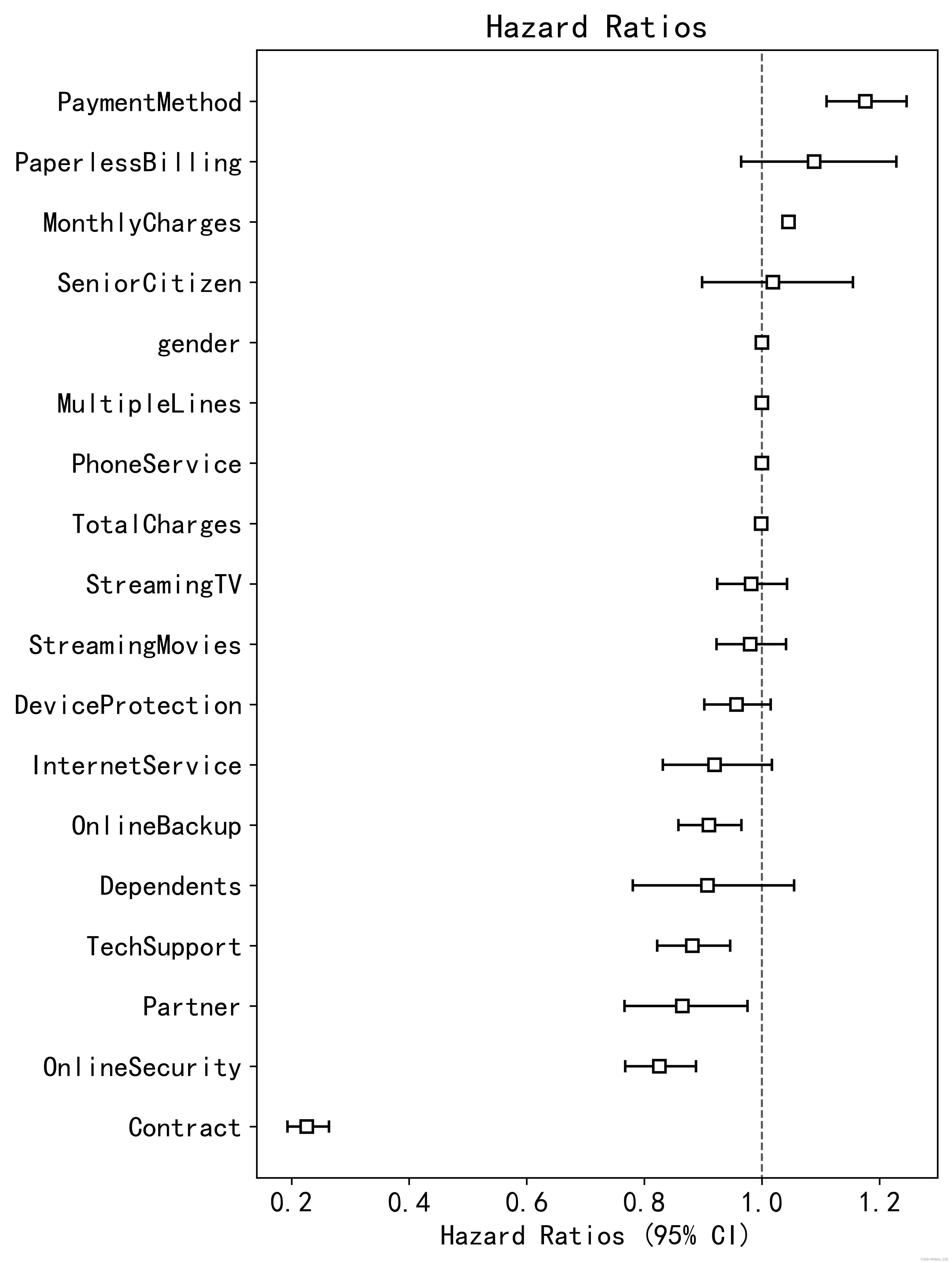
7、评估预测效果
一致性指数
plt.figure(figsize =(6,10),dpi=600)
model.plot(hazard_ratios=True)
plt.xlabel('Hazard Ratios (95% CI)')
plt.title('Hazard Ratios')
布里尔分数(Brier Score)
loss_dict ={}for i inrange(1,72):
    score = brier_score_loss(
        test_data['Churn'],1-np.array(model.predict_survival_function(test_data).loc[i]), pos_label=1)
    loss_dict[i]=[score]

loss_df = pd.DataFrame(loss_dict).T

fig, ax = plt.subplots(dpi=600)
ax.plot(loss_df.index, loss_df)
ax.set(xlabel='Prediction Time', ylabel='Calibration Loss', title='Cox PH Model Calibration Loss / Time')
plt.show()
![[外链图片转存失败,源站可能有防盗链机制,建议将图片保存下来直接上传(img-yR6wntQk-1666921386506)(output_27_0.png)]](https://img-blog.csdnimg.cn/85e8ffc46fa145a7ada0813aec2eff85.png)
从图上看,模型对于预测40个月内的用户流失效果很好。
校准曲线(Calibration)
plt.figure(figsize=(10,10),dpi=600)

ax = plt.subplot2grid((3,1),(0,0), rowspan=2)
ax.plot([0,1],[0,1],"k:", label="Perfectly calibrated")

probs =1-np.array(model.predict_survival_function(test_data).loc[7])

actual = test_data['Churn']
fraction_of_positives, mean_predicted_value = calibration_curve(actual, probs, n_bins=10, normalize=False)

ax.plot(mean_predicted_value, fraction_of_positives,"s-", label="%s"%("CoxPH",))
ax.set_ylabel("Fraction of positives")
ax.set_ylim([-0.05,1.05])
ax.legend(loc="lower right")
ax.set_title('Calibration plots (reliability curve)')
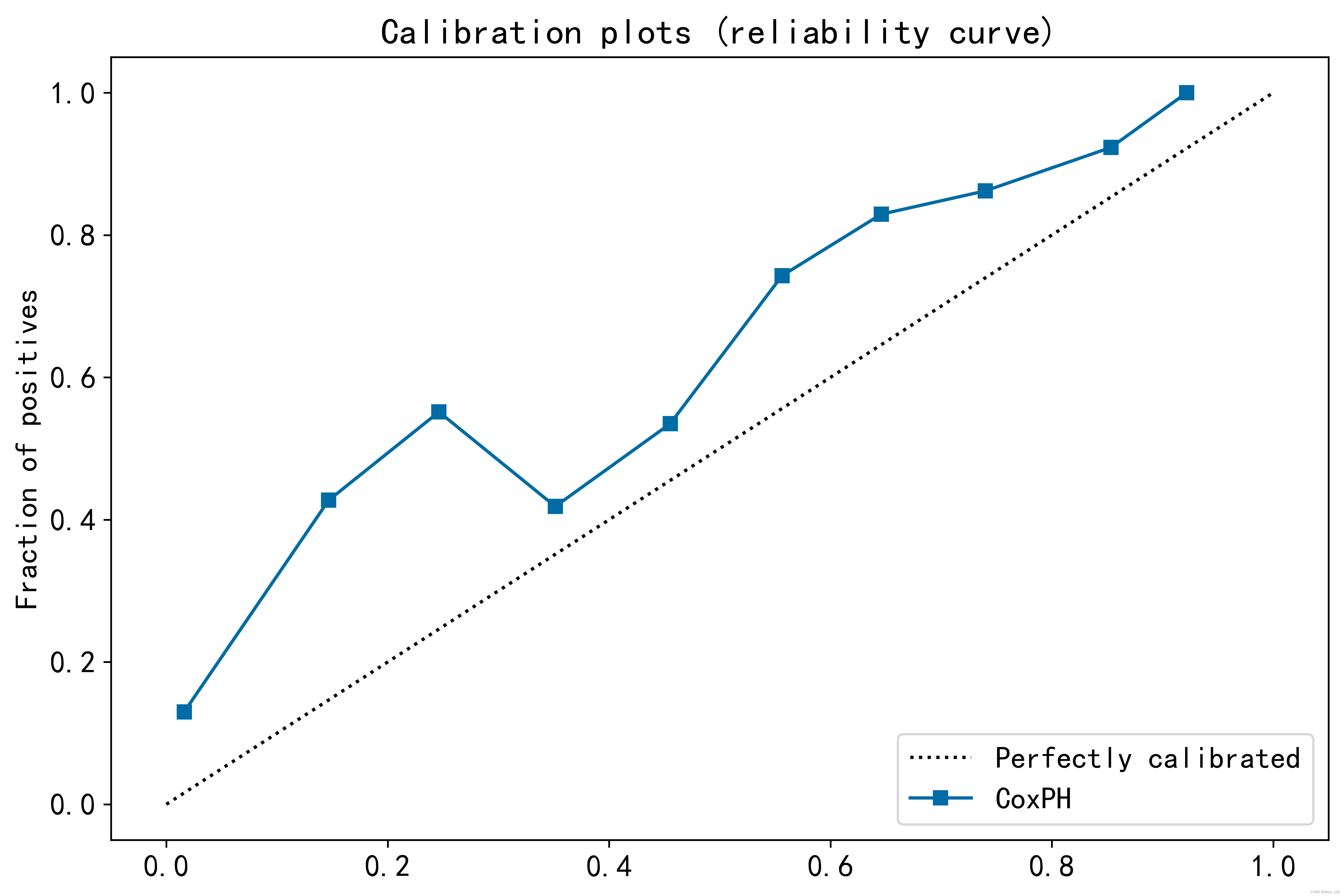
从图上看,模型低估了用户留存率,即高估了流失率。
8、预测抽样用户流失
nochurn_data=test_data.loc[test_data['Churn']==0]
churn_clients = pd.DataFrame(model.predict_survival_function(nochurn_data))
churn_clients
3943496261866761311538730152080544540952928637652308705422...21491380501421021106050293757715022190118852365974166813121.000.910.991.001.001.000.961.001.001.000.771.001.001.001.001.00...1.001.001.001.000.981.001.000.981.001.001.001.000.991.001.002.000.870.991.001.001.000.951.001.001.000.681.001.001.001.001.00...1.001.001.001.000.981.001.000.981.001.001.001.000.991.001.003.000.840.981.001.001.000.931.001.001.000.621.001.001.001.001.00...1.001.001.001.000.971.001.000.971.001.001.001.000.981.001.004.000.800.981.001.001.000.921.001.001.000.551.001.001.001.001.00...1.001.001.001.000.961.001.000.971.001.001.001.000.981.001.005.000.770.971.000.991.000.911.001.001.000.491.001.001.001.001.00...1.001.001.001.000.961.001.000.961.001.000.991.000.971.001.00................................................................................................68.000.000.000.060.030.200.000.970.990.960.001.000.800.971.000.98...0.320.940.980.600.000.740.900.001.000.410.030.200.000.090.5969.000.000.000.040.020.160.000.970.990.950.001.000.780.971.000.98...0.280.930.980.560.000.710.890.001.000.360.020.160.000.070.5570.000.000.000.010.000.090.000.960.980.940.000.990.710.960.990.97...0.180.910.970.460.000.640.860.001.000.260.010.080.000.030.4571.000.000.000.010.000.050.000.950.980.930.000.990.670.950.990.96...0.130.890.970.400.000.580.830.001.000.200.000.050.000.010.3972.000.000.000.000.000.040.000.950.980.920.000.990.630.950.990.96...0.100.880.960.350.000.540.810.001.000.160.000.030.000.010.34
72 rows × 1031 columns
plt.figure(figsize=(10,10),dpi=600)
churn_clients[churn_clients.columns[0]].plot(color='c')
churn_clients[churn_clients.columns[1]].plot(color='y')
churn_clients[churn_clients.columns[21]].plot(color='m')
churn_clients[1311].plot(color='g')
plt.plot([i for i inrange(0,20)],[0.5for i inrange(0,20)],'k--', label='Threshold=0.5')
plt.ylim(0,1)
plt.xlim(0,72)
plt.xlabel('Timeline')
plt.ylabel('Retain probability')
plt.legend(loc='best')
plt.title('The Churn Trend of Samples')
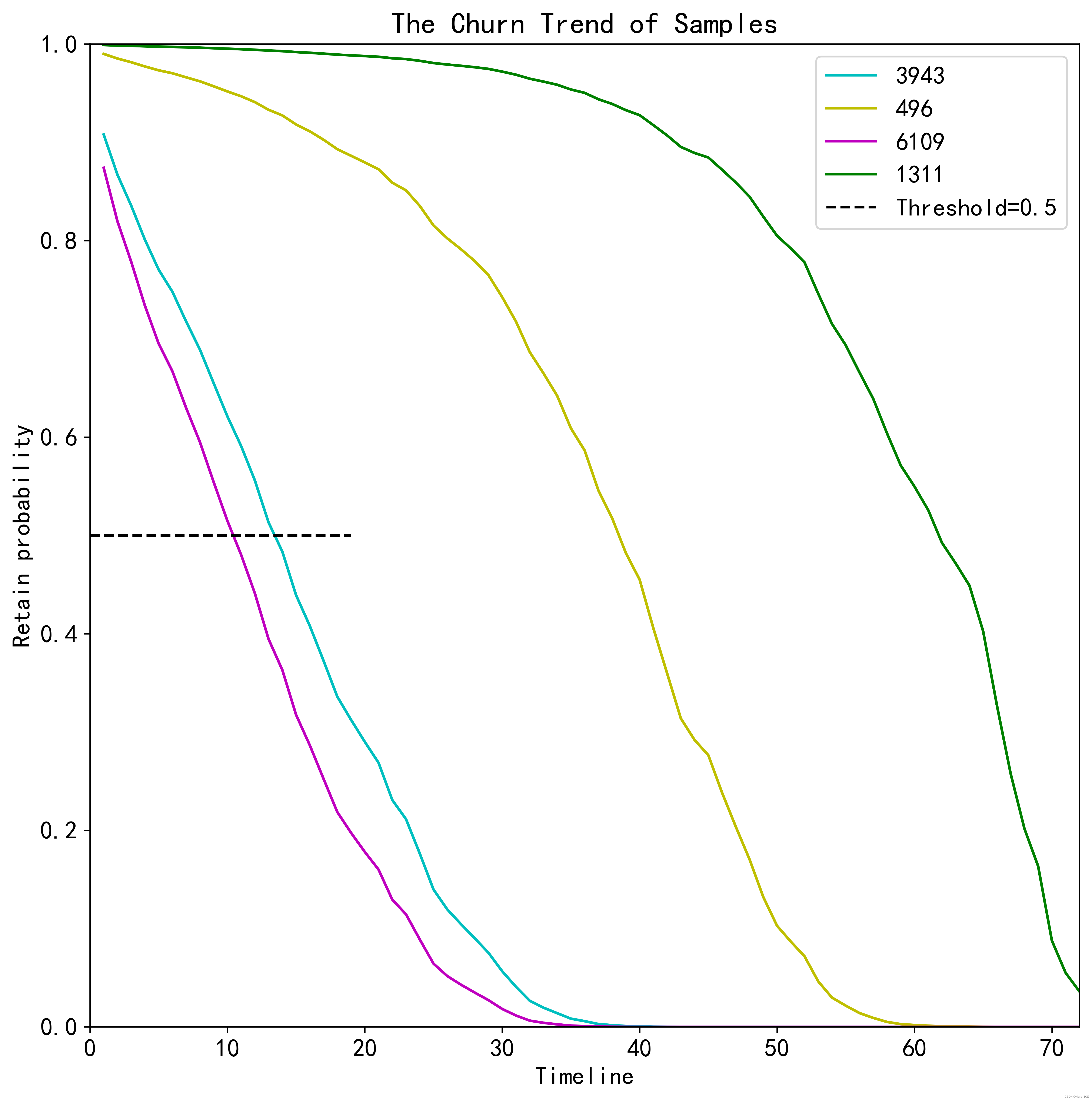
从图上看,序号为6109的用户在第10个月的时候,留存率开始低于50%,在第30个月和第40个月之间流失。
七、分层召回用户
基于上述分析,给出对于召回用户的如下建议:
1)根据用户流失风险等级划分用户,对于不同流失风险等级的客户,采用不用运营策略;
2)根据流失预测模型,要在合适的时间点进行干预,以最小的成本留住客户。
3)优化建议:提取其他数据,如用户消费数据,对用户价值分层,进一步精细化管理用户。
版权归原作者 Mars_1GE 所有, 如有侵权,请联系我们删除。