python机器学习_近邻算法_分类Ionosphere电离层数据

文章目录

摘要

本文使用python机器学习库Scikit-learn中的工具，以某网站电离层数据为案例，使用近邻算法进行分类预测。并在训练后使用K折交叉检验进行检验，最后输出预测结果及准确率。过程产生一系列直观的可视化图像。希望文章能够对大家有所帮助。祝大家学习顺利！

1.数据获取

1.点击链接获取数据
数据获取链接
http://archive.ics.uci.edu/ml/datasets/Ionosphere
2.点击Data Floder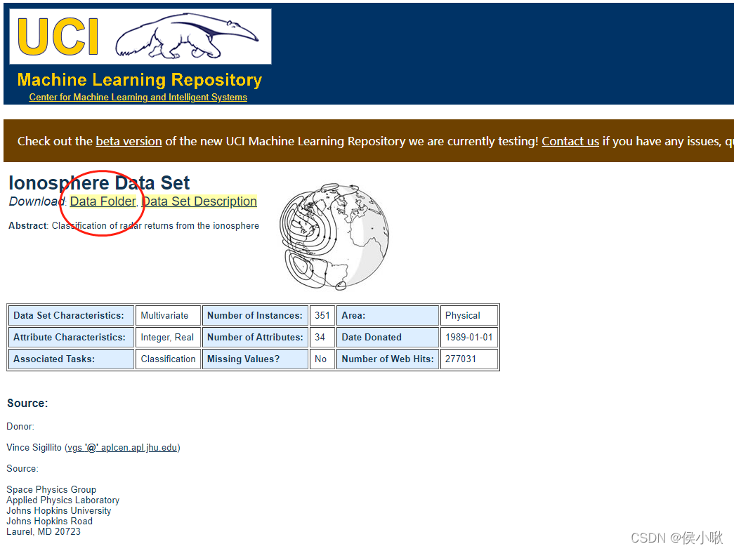

3.选择ionosphere.data和ionosphere.name这两个文件并下载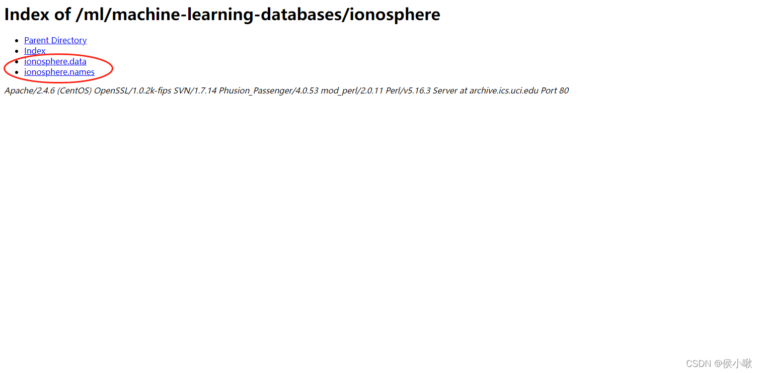

4.下载后放在指定目录下，可以直接通过pycharm查看数据的基本信息
ionosphere.data是我们需要用到的数据，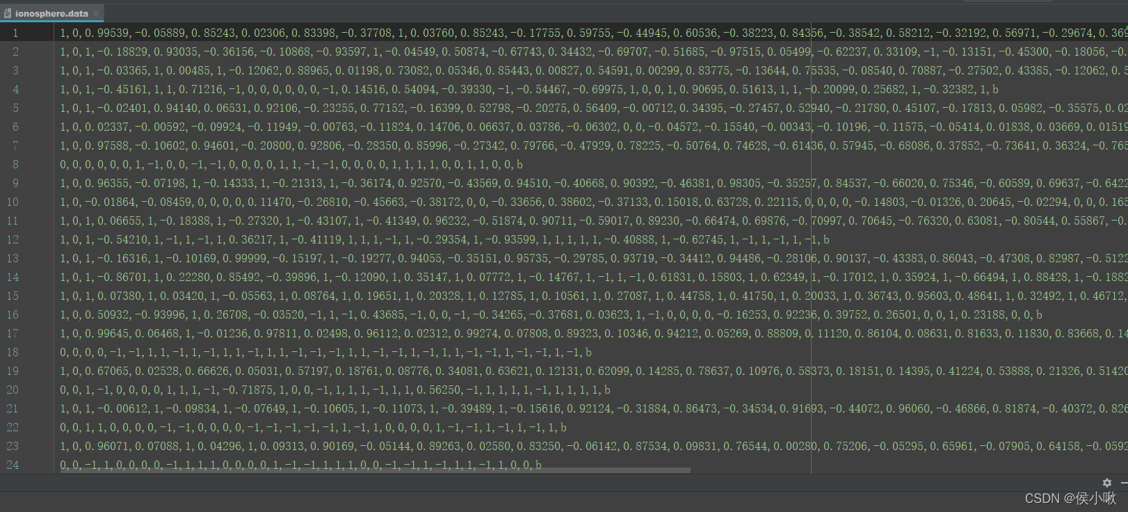

ionosphere.name是对该数据的介绍。

从ionosphere.name中可以看到，ionosphere.data共有351个样本，34个特征，且第35个表示类别，有g和b两个取值，分别表示“good”和“bad”。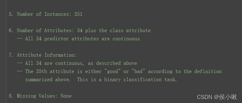

2.数据集分割与初步训练表现

import os
import csv
import numpy as np
from sklearn.model_selection import train_test_split
from sklearn.neighbors import KNeighborsClassifier
from sklearn.model_selection import cross_val_score
from matplotlib import pyplot as plt
from collections import defaultdict

data_filename ="ionosphere.data"

X = np.zeros((351,34), dtype='float')
y = np.zeros((351,), dtype='bool')withopen(data_filename,'r')as input_file:
    reader = csv.reader(input_file)# print(reader)  # csv.reader类型for i, row inenumerate(reader):
        data =[float(datum)for datum in row[:-1]]# Set the appropriate row in our dataset
        X[i]= data
        # 将“g”记为1，将“b”记为0。
        y[i]= row[-1]=='g'# 划分训练集、测试集
X_train, X_test, y_train, y_test = train_test_split(X, y, random_state=14)# 即创建估计器（K近邻分类器实例） 默认选择5个近邻作为分类依据
estimator = KNeighborsClassifier()# 进行训练，
estimator.fit(X_train, y_train)# 评估在测试集上的表现
y_predicted = estimator.predict(X_test)# 计算准确率
accuracy = np.mean(y_test == y_predicted)*100print("The accuracy is {0:.1f}%".format(accuracy))# 进行交叉检验，计算平均准确率
scores = cross_val_score(estimator, X, y, scoring='accuracy')
average_accuracy = np.mean(scores)*100print("The average accuracy is {0:.1f}%".format(average_accuracy))

如图，该分类算法准确率可达86.4%，交叉检验后的平均准确率可达82.6%。属于是比较优秀的算法。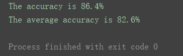

3.测试不同近邻值

测试不同的 近邻数 n_neighbors的值（上边默认为5）下的分类准确率，
选择近邻值从1到20的二十个数字，
并绘图展示

avg_scores =[]
all_scores =[]
parameter_values =list(range(1,21))# Including 20for n_neighbors in parameter_values:
    estimator = KNeighborsClassifier(n_neighbors=n_neighbors)
    scores = cross_val_score(estimator, X, y, scoring='accuracy')
    avg_scores.append(np.mean(scores))
    all_scores.append(scores)# 绘制n_neighbors的不同取值与分类正确率之间的关系
plt.figure(figsize=(32,20))
plt.plot(parameter_values, avg_scores,'-o', linewidth=5, markersize=24)
plt.show()

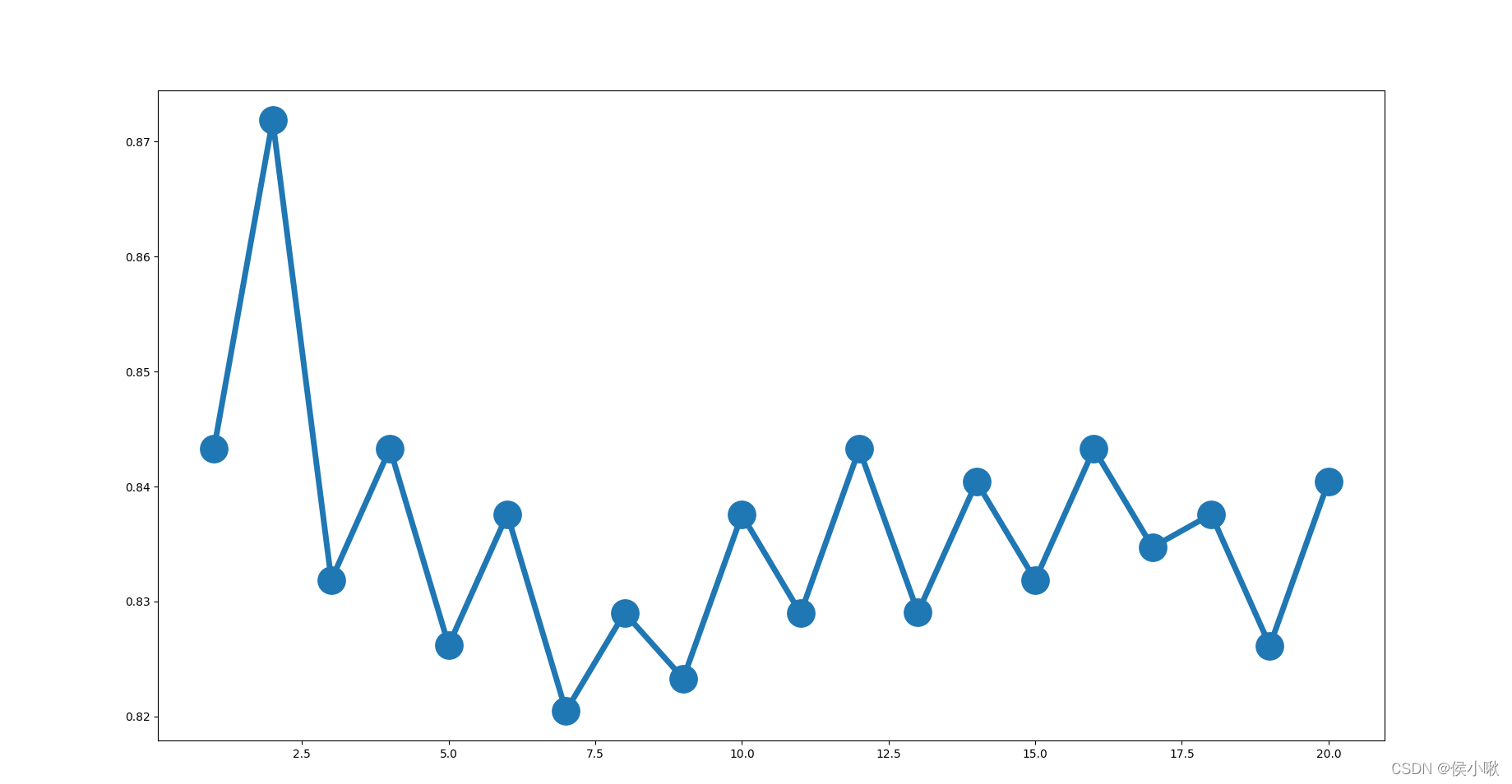
可以看出，准确率整体趋势随着近邻数的增加而减小。近邻值为2时准确率最高。

4.交叉检验

把交叉检验每次验证的准确率也绘制出来
（20个近邻值每个对应5个训练集，对应5次检验）

for parameter, scores inzip(parameter_values, all_scores):
    n_scores =len(scores)
    plt.plot([parameter]* n_scores, scores,'-o')
plt.show()

各次检验准确率图示如下：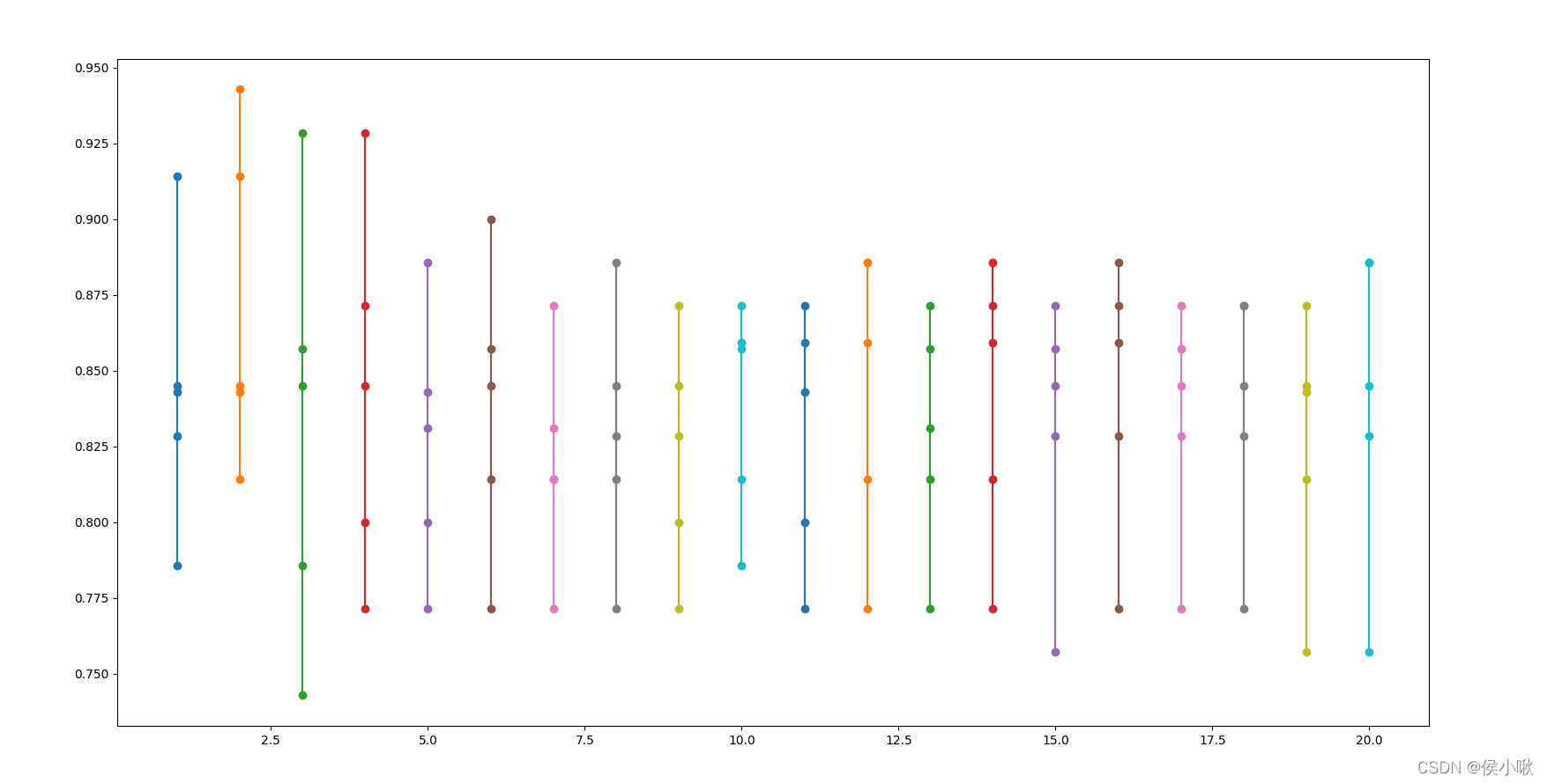

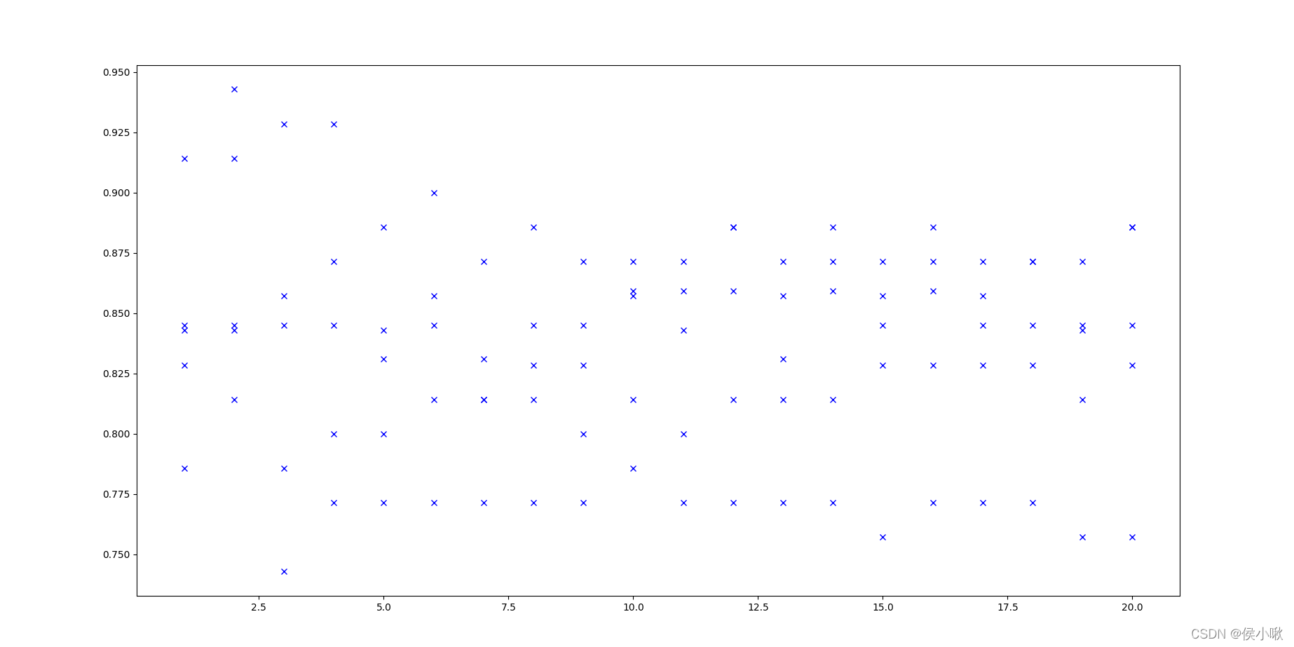
绘制出散点图

plt.plot(parameter_values, all_scores,'bx')
plt.show()

5. 十折交叉检验

all_scores = defaultdict(list)
parameter_values =list(range(1,21))# Including 20for n_neighbors in parameter_values:
    estimator = KNeighborsClassifier(n_neighbors=n_neighbors)
    scores = cross_val_score(estimator, X, y, scoring='accuracy', cv=10)
    all_scores[n_neighbors].append(scores)for parameter in parameter_values:
    scores = all_scores[parameter]
    n_scores =len(scores)
    plt.plot([parameter]* n_scores, scores,'-o')  

plt.plot(parameter_values, avg_scores,'-o')
plt.show()

检验结果如下图所示：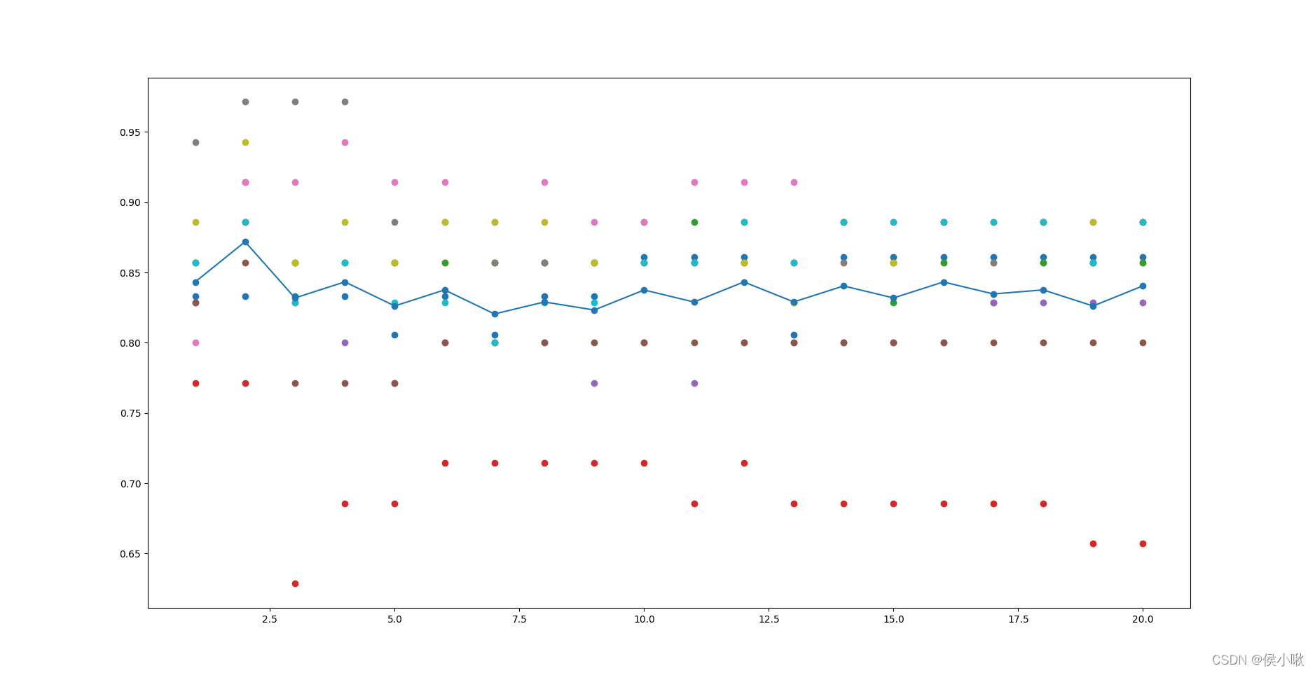

因为每个近邻值下，10次检验中的准确率可能会有重复值，所以在图像中每个近邻值上的准确率个数会有差异。

6.输出预测结果

这里用测试集作为待测数据，使用上述算法进行预测，并输出预测结果，
且令n_neighbors=2

Estimator = KNeighborsClassifier(n_neighbors=2)
Estimator.fit(X_train, y_train)
Y_predicted = Estimator.predict(X_test)
accuracy = np.mean(y_test == Y_predicted)*100
pre_result = np.zeros_like(Y_predicted, dtype=str)
pre_result[Y_predicted ==1]='g'
pre_result[Y_predicted ==0]='b'print(pre_result)print("The accuracy is {0:.1f}%".format(accuracy))

程序运行结果如下：

如图，预测准确率达92.0%。