LLM - LLaMA-2 获取文本向量并计算 Cos 相似度

一.引言

前面提到了两种基于统计的机器翻译评估方法: Rouge 与 BLEU，二者通过统计概率计算 N-Gram 的准确率与召回率，在机器翻译这种回答相对固定的场景该方法可以作为一定参考，但在当前大模型更加多样性的场景以及发散的回答的情况下，Rouge 与 BLEU 有时候并不能更好的描述文本之间的相似度，下面我们尝试从 LLM 大模型提取文本的 Embedding 并进行向量相似度计算。

二.获取文本向量

1.hidden_states 与 last_hidden_states

根据 LLM 模型类型的不同，有的 Model 提供 hidden_states 方法，例如 LLaMA-2-13B，有的模型提供 last_hidden_states 方法，例如 GPT-2。查找模型对应方法 API 可以在 Transformer 官网。

◆** hidden_states**

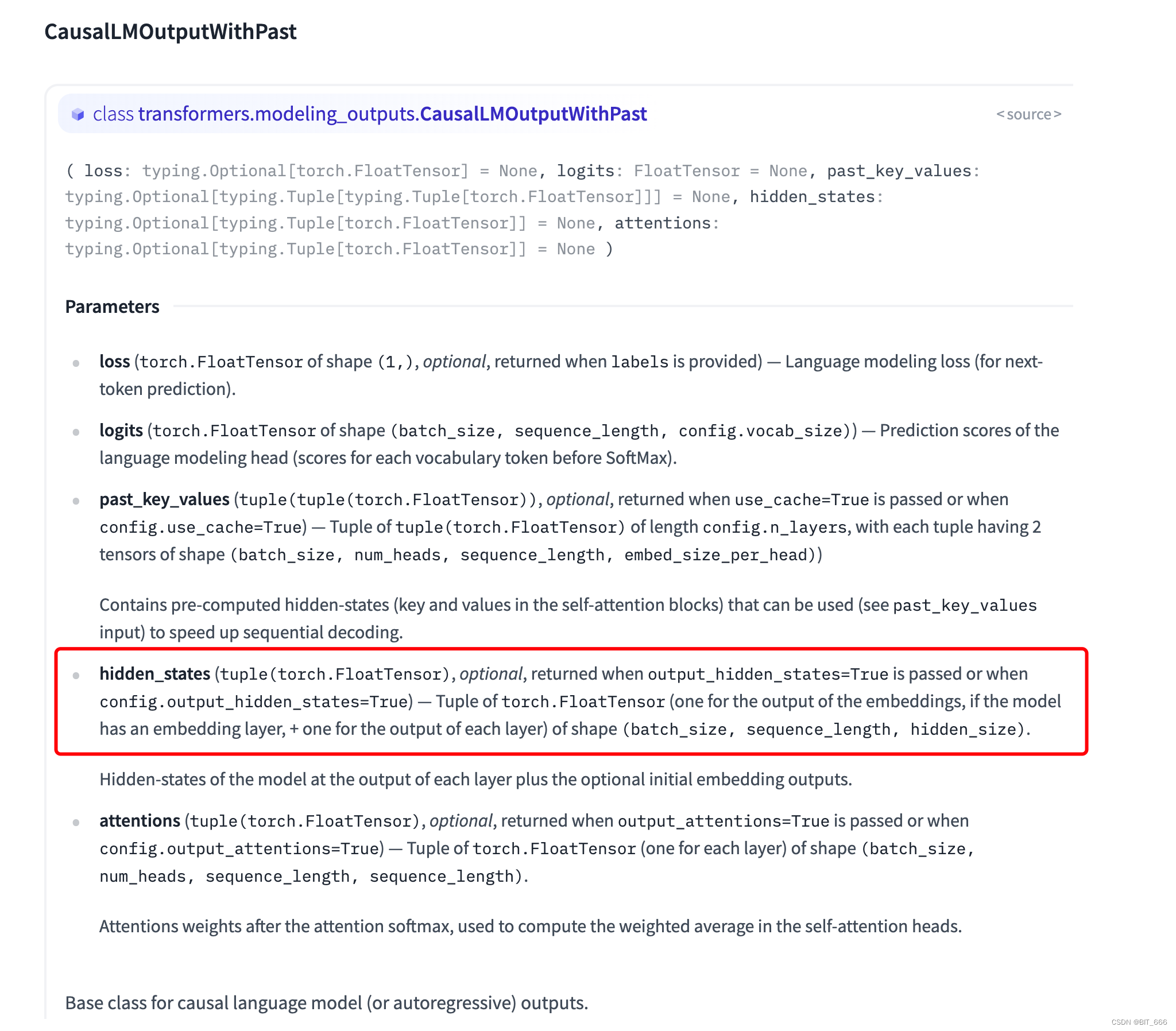
hidden_states 类型为 typing.Optional[typing.Tuple[torch.FloatTensor]]，其提供一个 Tuple[Tensor] 分别记录了每层的输出，完整的解释在参数下方:

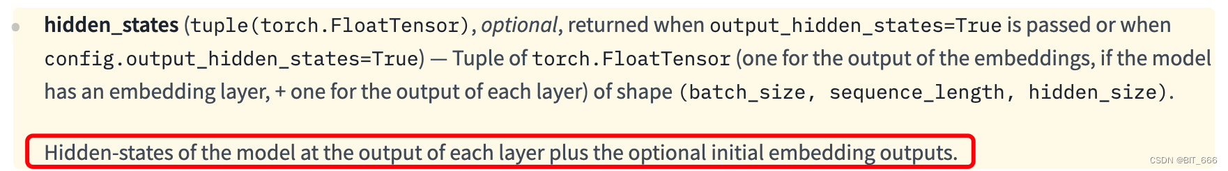
模型在每一层输出处的隐藏状态加上可选的初始嵌入输出。这里我们可以通过打印模型 Layer 和索引从而获取 hidden_states 中隐层的输出。

***◆ *last_hidden_states **

一些传统的模型例如 GPT-2，还有当下一些的新模型例如 ChatGLM2 都有 last_hidden_states 的 API，可以直接获取最后一层的 Embedding 输出，而如果使用 hidden_states 则只需要通过 [-1] 索引即可获得 last_hidden_states，相比来如前者更全面后者更方便。

2.LLaMA-2 获取 hidden_states

***◆ *model config **

    config_kwargs = {
        "trust_remote_code": True,
        "cache_dir": None,
        "revision": 'main',
        "use_auth_token": None,
        "output_hidden_states": True
    }

    config = AutoConfig.from_pretrained(ori_model_path, **config_kwargs)

    llama_model = AutoModelForCausalLM.from_pretrained(
        ori_model_path,
        config=config,
        torch_dtype=torch.float16,
        low_cpu_mem_usage=True,
        trust_remote_code=True,
        revision='main'
    )

根据 CausalLMOutputWithPast hidden_states 参数的提示，我们只需要在模型 config 中添加:

"output_hidden_states": True

◆ get Embedding

def get_embeddings(result, llm_tokenizer, model, args):
    fw = open(args.output, 'w', encoding='utf-8')
    for qa in result:
        q = qa[0]
        a = qa[1]
        # 对输出文本进行 tokenize 和编码
        tokens = llm_tokenizer.encode_plus(a, add_special_tokens=True, padding='max_length', truncation=True,
                                           max_length=128, return_tensors='pt')
        input_ids = tokens["input_ids"]
        attention_mask = tokens['attention_mask']

        # 获取文本 Embedding
        with torch.no_grad():
            outputs = model(input_ids=input_ids.cuda(), attention_mask=attention_mask)
            embedding = list(outputs.hidden_states)
            last_hidden_states = embedding[-1].cpu().numpy()
            first_hidden_states = embedding[0].cpu().numpy()
            last_hidden_states = np.squeeze(last_hidden_states)
            first_hidden_states = np.squeeze(first_hidden_states)
            fisrt_larst_avg_status = np.mean(first_hidden_states + last_hidden_states, axis=0)

        log = "%s\t%s\t%s\n" % (q, a, toString(fisrt_larst_avg_status))
        fw.write(log)
    fw.close()

predict 预测 ➔ 将 model 基于 Question generate 得到的 Answer 存入 result

encode 编码 ➔ 对 Answer 进行编码获取对应 Token 与 input_ids、attention_mask

output 模型输出 ➔ 直接调用 model 进行输出，有的也可以调用 model.transform 方法进行输出

hidden_states ➔ outputs.hidden_states 获取各隐层输出

最后获取的向量需要先 cpu 然后再转为 numpy 数组，一般的做法是采用 mean 获得句子的平均表征。

三.获取向量 Cos 相似度

1.向量选择

在 BERT-flow 的论文中，如果不加任何后处理手段，那么基于 BERT 抽取句向量的最好 Pooling 方法是 BERT 的第一层与最后一层的所有 token 向量的平均，即 fisrt-larst-avg，对应 hidden_state 的 0 和 -1 索引，所以后面的相似度计算我们都以 fisrt-larst-avg 为基准来评估 Embedding 相似度。

# 获取文本 Embedding
with torch.no_grad():
    outputs = model(input_ids=input_ids.cuda(), attention_mask=attention_mask)
    embedding = list(outputs.hidden_states)
    last_hidden_states = embedding[-1].cpu().numpy()
    first_hidden_states = embedding[0].cpu().numpy()
    last_hidden_states = np.squeeze(last_hidden_states)
    first_hidden_states = np.squeeze(first_hidden_states)
    fisrt_larst_avg_status = np.mean(first_hidden_states + last_hidden_states, axis=0)

2.Cos 相似度

# 计算 Cos 相似度
def compute_cosine(a_vec, b_vec):
    norms1 = np.linalg.norm(a_vec, axis=1)
    norms2 = np.linalg.norm(b_vec, axis=1)
    dot_products = np.sum(a_vec * b_vec, axis=1)
    cos_similarities = dot_products / (norms1 * norms2)
    return cos_similarities

a_vec 为预测文本转化得到的 Embedding，b_vec 为人工标注正样本文本转化得到的 Embedding，通过计算二者相似度，评估预测文本与人工文本的相似程度。

3.BERT-whitening 特征白化

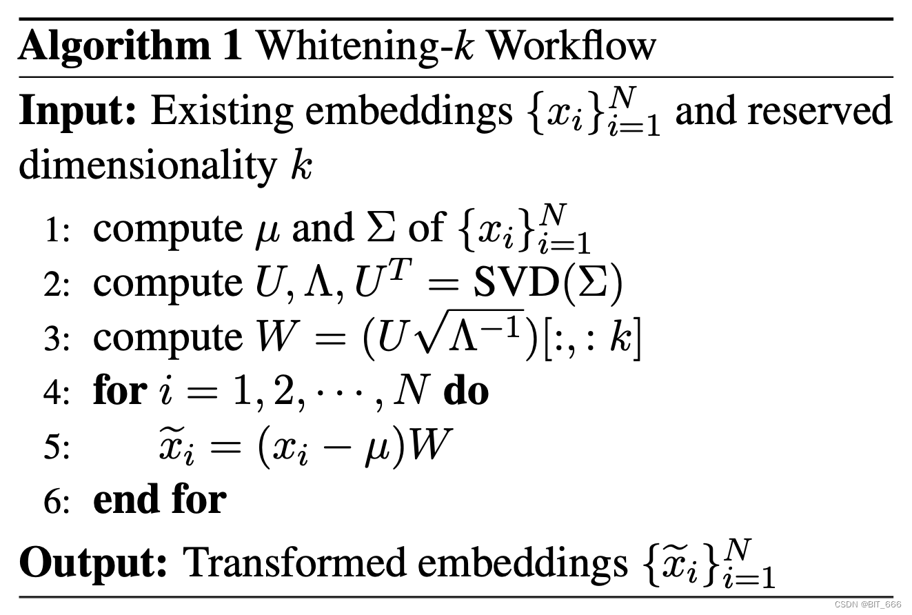
苏神在 BERT-whitening 一文中提出了一种基于 PCA 降维的无监督 Embedding 评估方式，Bert-whitening 又叫特征白化，其思路与 PCA 降维类似，意在对 SVD 分解后的主成分矩阵取前 λ 个特征向量构造特征值矩阵，提取向量中的关键信息，使输出向量矩阵每个维度均值为零，协方差矩阵为单位阵，λ 个特征值也对应前 λ 个主成分。其算法逻辑如下：

下面我们调用 Sklearn 的 PCA 库简单实现下:

from sklearn.decomposition import PCA
from sklearn.preprocessing import normalize

    # 取出句子的平均表示 -> 使用 PCA 降维 -> 白化处理
    concatenate = np.concatenate((answer_vector, predict_vector))
    pca = PCA(n_components=2048)
    pca.fit(concatenate)
    ans_white_vec = pca.transform(answer_vector)
    ans_norm_vec = normalize(ans_white_vec)
    pre_white_vec = pca.transform(predict_vector)
    pre_norm_vec = normalize(pre_white_vec)

    pca_cos_similarities = compute_cosine(ans_norm_vec, pre_norm_vec)

answec_vector 和 predict_vector 均通过 first_and_last 方法从 hidden_states 中获取，n_components 即 top_k 的选择，以 LLaMA-2 为例，原始得到的向量维度为 5120，原文中也有使用 n_components = 256 实验。

4.评估指标对比

在同一份标准答案的基础上，博主分别使用 LLaMA-33B、LLaMA-2-13B、Aplace-2-13B 进行了向量相似度的指标评估，肉眼看效果 LLaMA-33B > LLaMA-2-13B > Aplace-2-13B，实际的指标也基本保持了这个趋势：

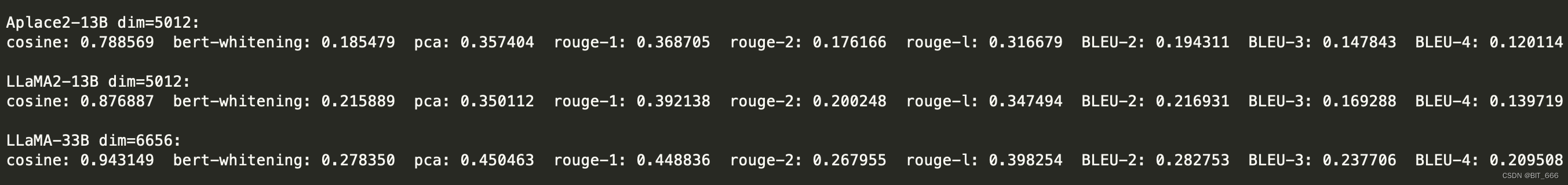
一方面 LLaMA-33B 凭借参数量和 Embedding 维度的优势保持了各项指标的领先，其次回归到这些相似度评估指标身上，Embedding 层得到的 First Layer 其实是 Token 的表征，而 Last Layer 得到的是 Next Token 的分布，不管基于 COS 还是 PCA，这些指标还是没有脱离 Rouge、Bleu 的统计概率，只不过是更加抽象的文本相似。想要做到更深层次的语义理解，可以需要有监督样本训练后的 LLM 去评估，不过起码现在有了除 Rouge、Bleu 外的指标了。

四.总结

博主采用 1500+ 样本分别使用 cos、pca 和 self_pca [自己实现 SVD 与特征矩阵] 三种方法对向量相似度进行评估，n_components 设为 1024：

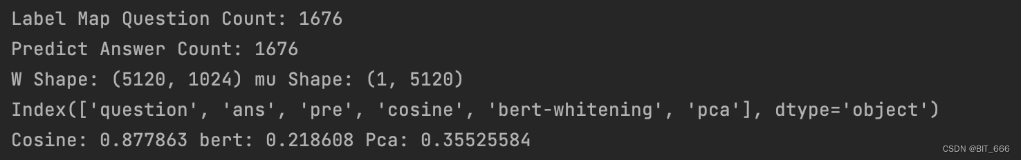
可以看到 SVD 处理后得到的 W 和 mu 的 shape，通过下述操作可完成向量的降维：

vecs = (vecs + bias).dot(kernel)

最终得到的结果 Cosine 与 PCA 降维的相似度差距较大，由于自然语言生成的样本没有严格意义的正样本，上面计算采用的参考文本也是人工标注，有一定的不确定性，所以基于不同的度量，我们也可以统计分析，定一个 threshold，认为大于该 threshold 的输入样本为可用。

Tips:

what is your name? => 'what' 'is' 'your' 'name' '?'
你的名字是什么? => '你' '的' '名' '字' '是' '什' '么' '?'

以上面的语句为例，如果是英文分词可以将每个词分解开，但是中文的词一定程度上需要用到词组，虽然 Rouge 可以计算 N-Gram 也可以覆盖一部分词组，但是整体意思还是有偏差，所以有兴趣的同学也可以尝试将逐字分词修改为 jieba 分词等，查看指标是否有变化：

你的名字是什么? => '你' '的' '名字' '是' '什么' '?'