深度学习05——线性回归模型

1.线性回归概述及其简单实现

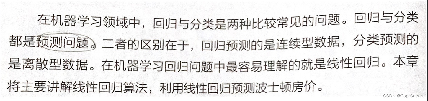
1.1 Numpy实现线性回归

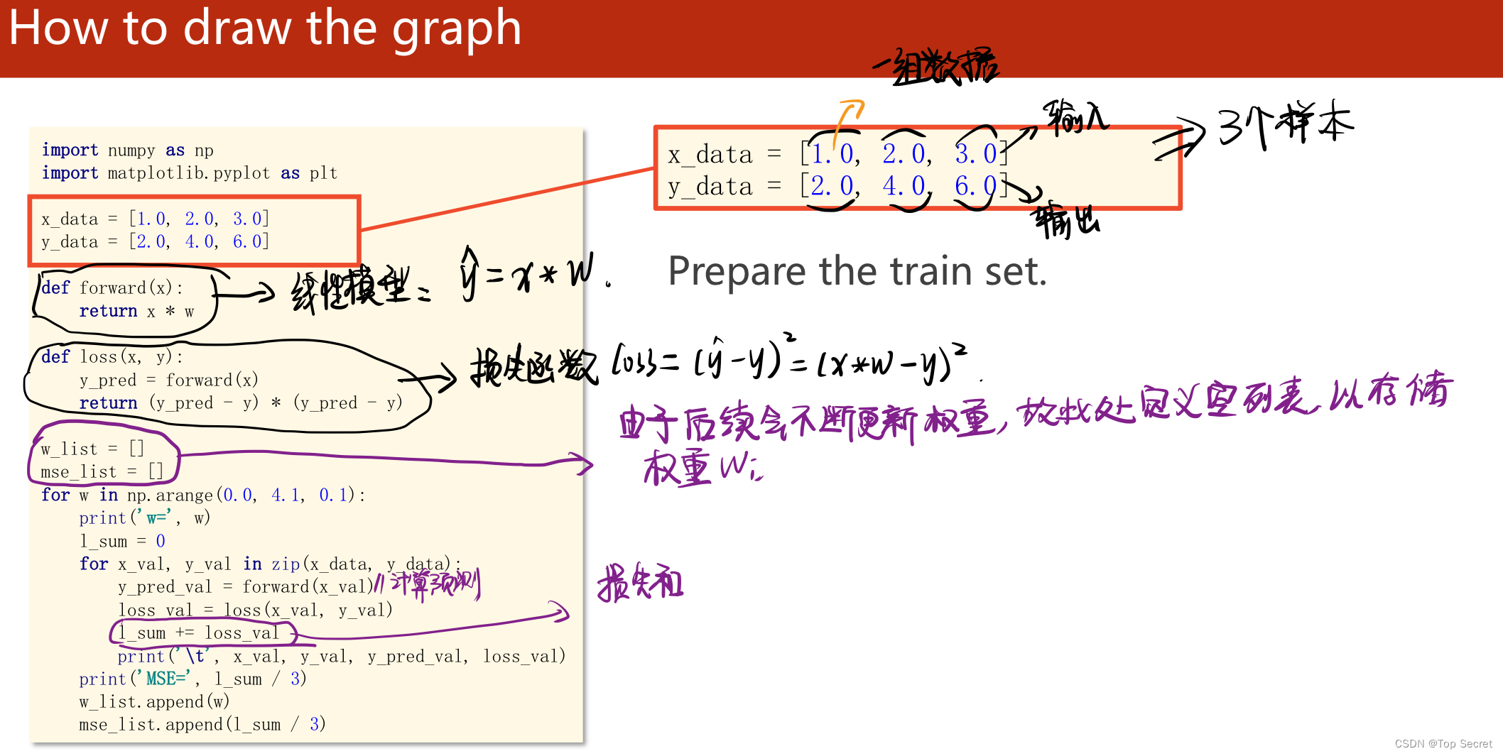
1.1.1 穷举法更新参数w，模型y = w*x

传送门

import numpy as np
import matplotlib.pyplot as plt

#写入数据集
x_data = [1.0, 2.0, 3.0]
y_data = [2.0, 4.0, 6.0]

# 线性回归模型
def forward(x):
    return x * w

#计算损失函数（MSE均方误差）
def loss(x, y):
    y_pred = forward(x)
    return (y_pred - y) ** 2

# 穷举法更新参数w
w_list = [] #用于存放更新的参数w
mse_list = []
for w in np.arange(0.0, 4.1, 0.1):
    print("w=", w)
    l_sum = 0  # 初始化，用于计算损失和
    for x_val, y_val in zip(x_data, y_data):
        y_pred_val = forward(x_val)
        loss_val = loss(x_val, y_val)
        l_sum += loss_val # 计算损失和
        print('\t', x_val, y_val, y_pred_val, loss_val)
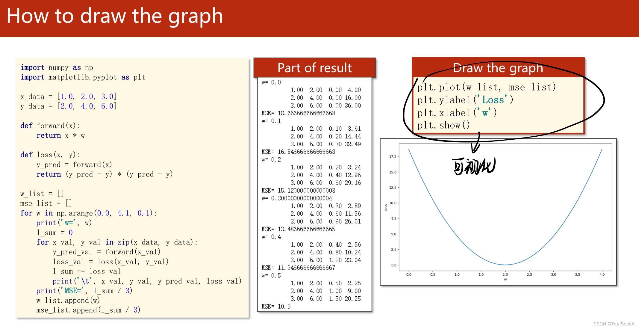
    print('MSE=', l_sum / 3)  #求均方误差
    w_list.append(w)  #将每一步更新的参数w存入列表w_list中，以便在后面可视化中绘制跟踪曲线
    mse_list.append(l_sum / 3)  

plt.plot(w_list, mse_list) #将参数w更新以及每一步计算损失函数的过程绘制出一个“跟踪曲线来”
plt.ylabel('Loss')
plt.xlabel('w')
plt.show()

代码助解：

​

​

注意：

(1) 如上代码的线性模型是：y = w*x

(2) python中zip()函数的用法:

传送门

zip函数的原型为：zip([iterable, …])：

参数iterable为可迭代的对象，并且可以有多个参数。该函数返回一个以元组为元素的列表，其中第 i 个元组包含每个参数序列的第 i 个元素。返回的列表长度被截断为最短的参数序列的长度。只有一个序列参数时，它返回一个1元组的列表。没有参数时，它返回一个空的列表。

import numpy as np
a=[1,2,3,4,5]
b=(1,2,3,4,5)
c=np.arange(5)
d="zhang"
zz=zip(a,b,c,d)
print(zz)

输出：
[(1, 1, 0, 'z'), (2, 2, 1, 'h'), (3, 3, 2, 'a'), (4, 4, 3, 'n'), (5, 5, 4, 'g')]

1.1.2 模型 y = w*x + b 实战

好文传送

# 使用模型y=wx+b，并绘制三维图形
import numpy as np
import matplotlib.pyplot as plt  # 绘图包

x_data = [1.0, 2.0, 3.0]  # 数据集保存，x和y需分开，x为输入，y为输出
y_data = [3.0, 5.0, 7.0]

def forward(x):  # 线性模型（前馈）
    return x * W + B  #加入偏置B

def loss(x, y):  # 损失函数
    y_pred = forward(x)
    return (y_pred - y) * (y_pred - y)

#更新参数w,B
w = np.arange(0.0, 4.1, 0.1)
b = np.arange(0.0, 2.1, 0.1)
[W, B] = np.meshgrid(w, b)  # 将w,b变为二维矩阵，将w和b变为二维矩阵后就不需要使用for循环来修改w的值

l_sum = 0

for x_val, y_val in zip(x_data, y_data):
    y_pred_val = forward(x_val)
    loss_val = loss(x_val, y_val)
    l_sum += loss_val
    print('\t', x_val, y_val, y_pred_val, loss_val)
print('MSE=', l_sum / 3)
# 此部分代码与例题完全相同，即使用forward函数计算x对应的y，用loss函数计算损失函数，MSE为平均损失函数

# 绘图：二维时使用plt.plot绘图，三维则使用matplotlib绘图
fig = plt.figure()
ax = fig.add_subplot(projection='3d')
# 引入3d绘图

ax.plot_surface(W, B, l_sum / 3)  # 引入W,B,l_sum/3三个绘图参数
plt.show()
# 引入matplotlib中的三维曲面图

输出：

​​

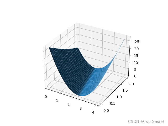
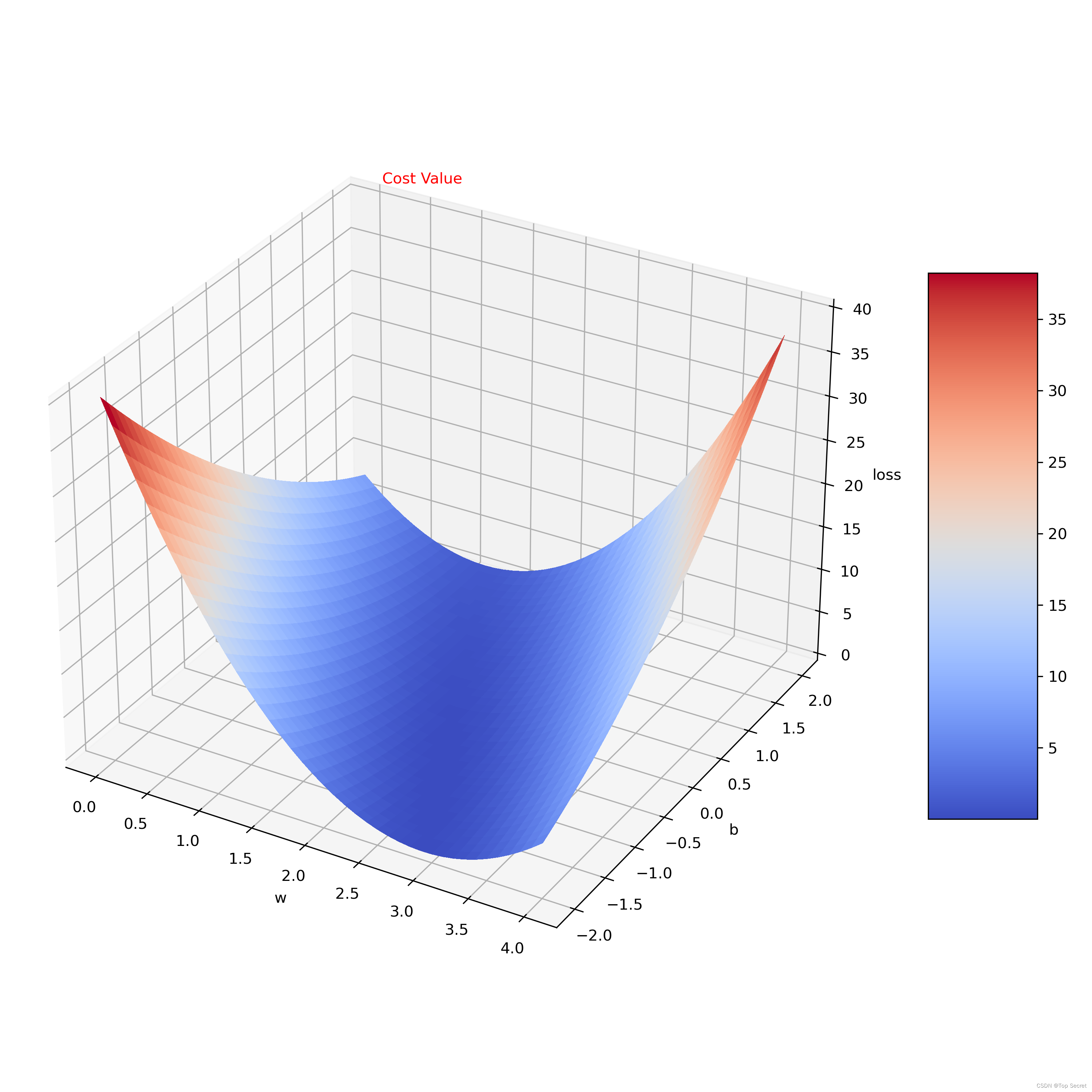
分析：此处代码的不同点在于第一个模型y=wx只需要更新参数w，而模型y=wx+b需要更新权重w和偏置b;还有需要注意的就是绘图时的差异。

1.1.3 对模型y = w*x 的代码实现（利用批量梯度下降）

​

​

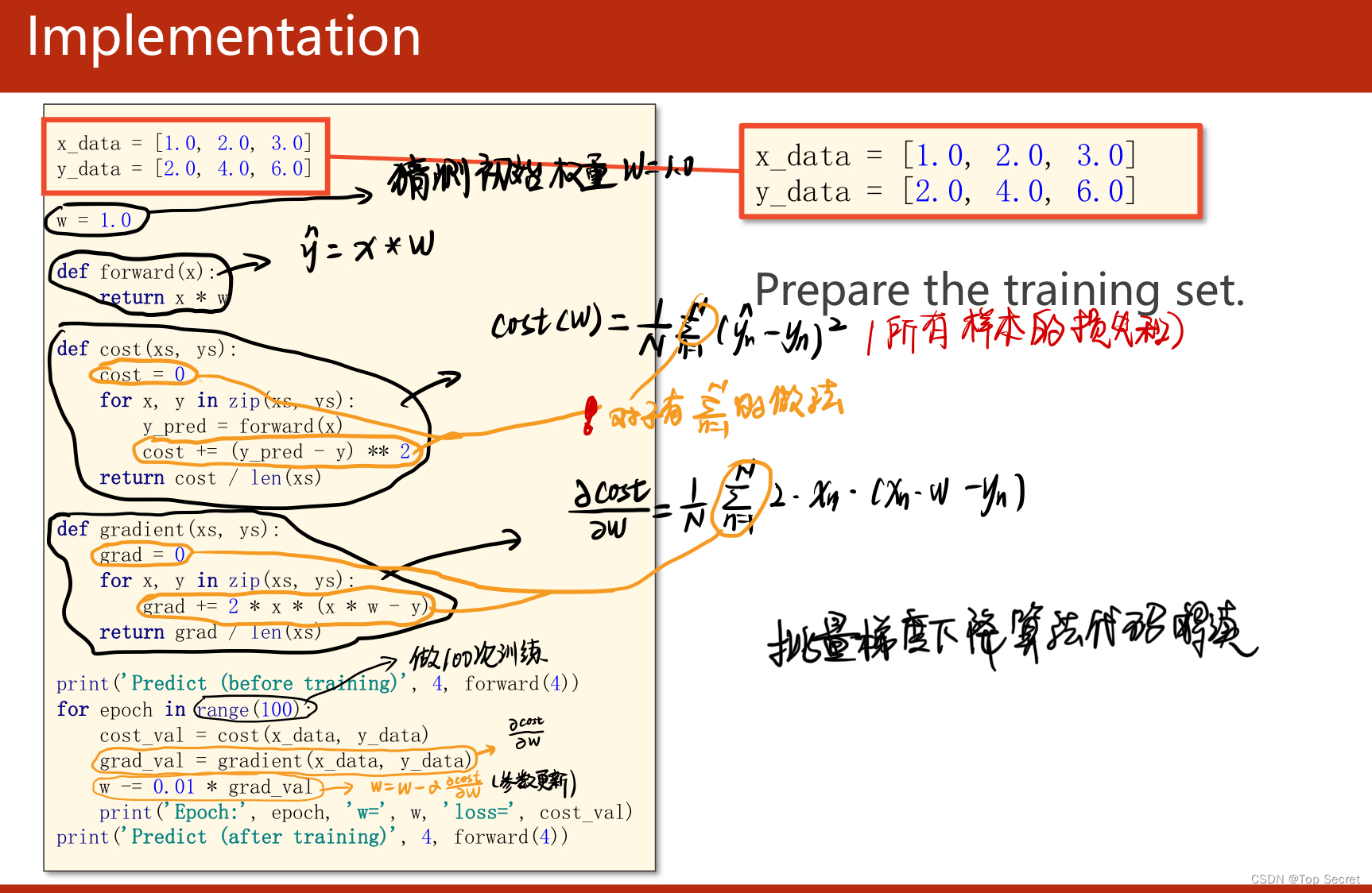
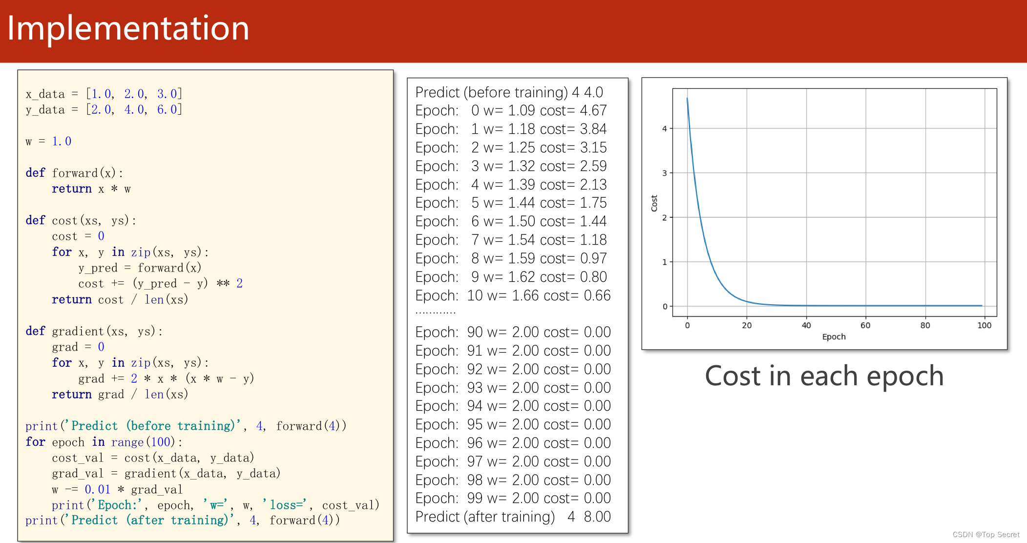
1.1.4 代码实现

import matplotlib.pyplot as plt

# prepare the training set
#准备数据集
x_data = [1.0, 2.0, 3.0]
y_data = [2.0, 4.0, 6.0]

# initial guess of weight
w = 1.0

# define the model linear model y = w*x
def forward(x):
    return x * w

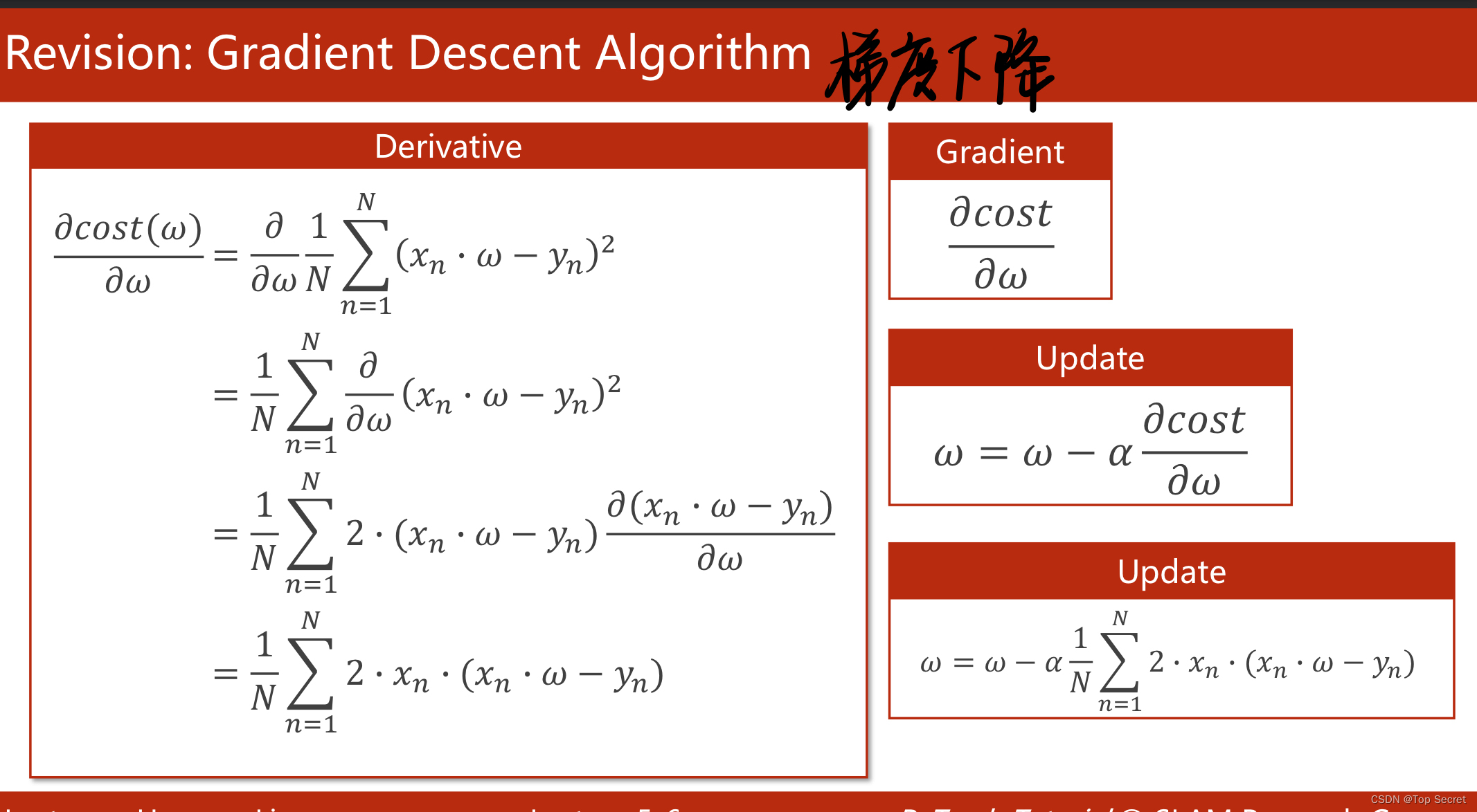
# define the cost function MSE
def cost(xs, ys):
    cost = 0
    for x, y in zip(xs, ys):
        y_pred = forward(x)
        cost += (y_pred - y) ** 2
    return cost / len(xs)

# define the gradient function  gd
def gradient(xs, ys):
    grad = 0
    for x, y in zip(xs, ys):
        grad += 2 * x * (x * w - y)
    return grad / len(xs)

epoch_list = []
cost_list = []
print('predict (before training)', 4, forward(4))
for epoch in range(100):
    cost_val = cost(x_data, y_data)  #caculate the sum of cost
    grad_val = gradient(x_data, y_data) # caculate the gradient
    w -= 0.01 * grad_val  # 0.01 learning rate
    print('epoch:', epoch, 'w=', w, 'loss=', cost_val)
    #将每次训练更新的的损失存入列表中
    epoch_list.append(epoch)
    cost_list.append(cost_val)

print('predict (after training)', 4, forward(4))
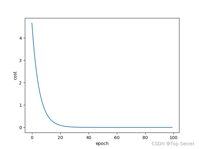
plt.plot(epoch_list, cost_list)
plt.ylabel('cost')
plt.xlabel('epoch')
plt.show()

运行结果:

​

2.1 又一个线性回归的实例（学习于龙老师）

# 实现一个线性回归的问题
# y = wx + b

step1: 计算损失函数loss的值

​

​

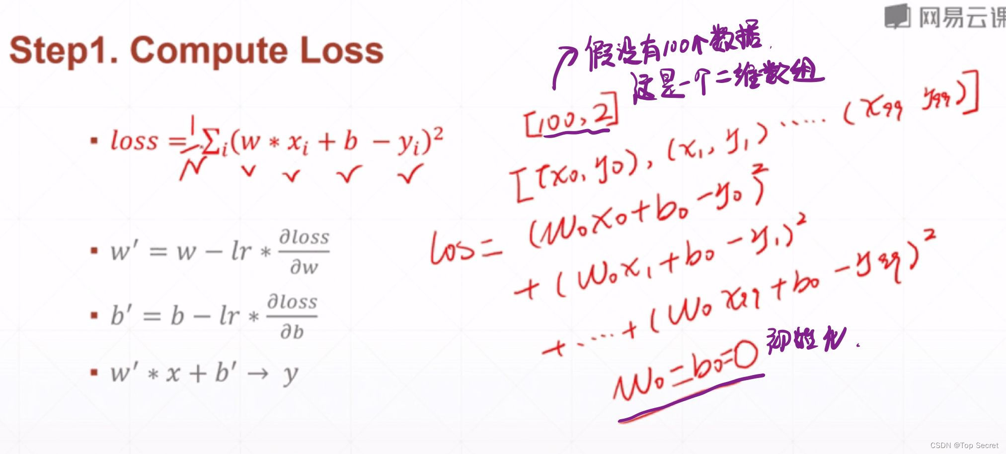
# 实现一个线性回归的问题
# y = wx + b
# step1: 计算损失函数loss的值
def compute_error_for_line_given_points(b, w, points):  #points表示数据的数量
    totalError = 0   #初始化损失函数的值
    for i in range(0, len(points)):
        x = points[i, 0]
        y = points[i, 1]
        # computer mean-squared-error
        totalError += (y - (w * x + b)) ** 2   #求loss的累积和
    # average loss for each point
    return totalError / float(len(points))

step2:计算梯度与更新

​

​

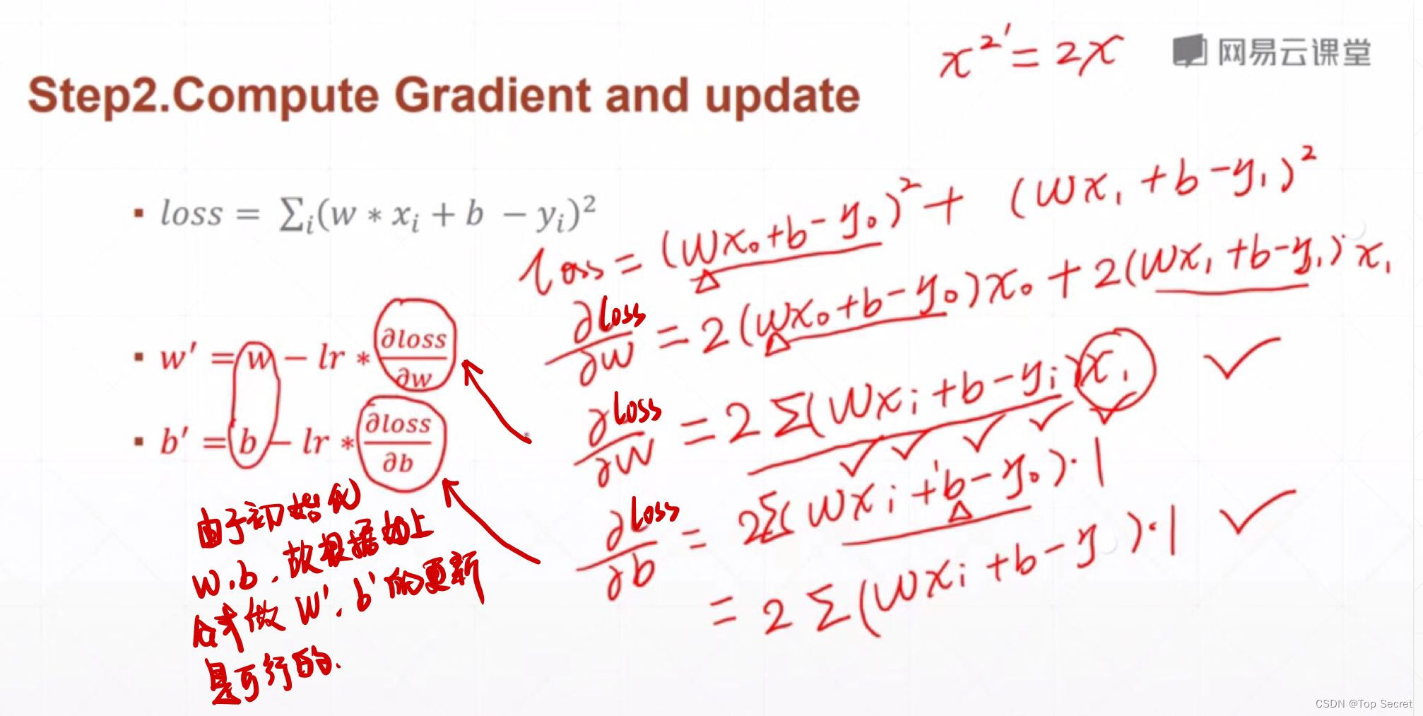
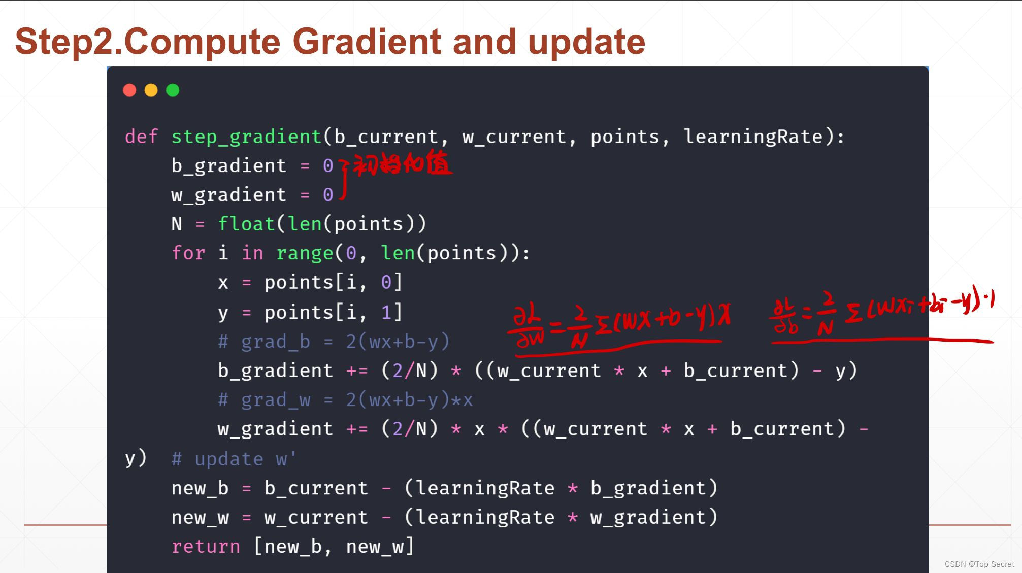
# step2:计算梯度与更新
def step_gradient(b_current, w_current, points, learningRate):
    b_gradient = 0
    w_gradient = 0
    N = float(len(points))
    for i in range(0, len(points)):
        x = points[i, 0]
        y = points[i, 1]
        # grad_b = 2(wx+b-y)
        b_gradient += (2/N) * ((w_current * x + b_current) - y)
        # grad_w = 2(wx+b-y)*x
        w_gradient += (2/N) * x * ((w_current * x + b_current) - y)
    # update w'
    new_b = b_current - (learningRate * b_gradient)
    new_w = w_current - (learningRate * w_gradient)
    return [new_b, new_w]

step3:更新权值w

​

​

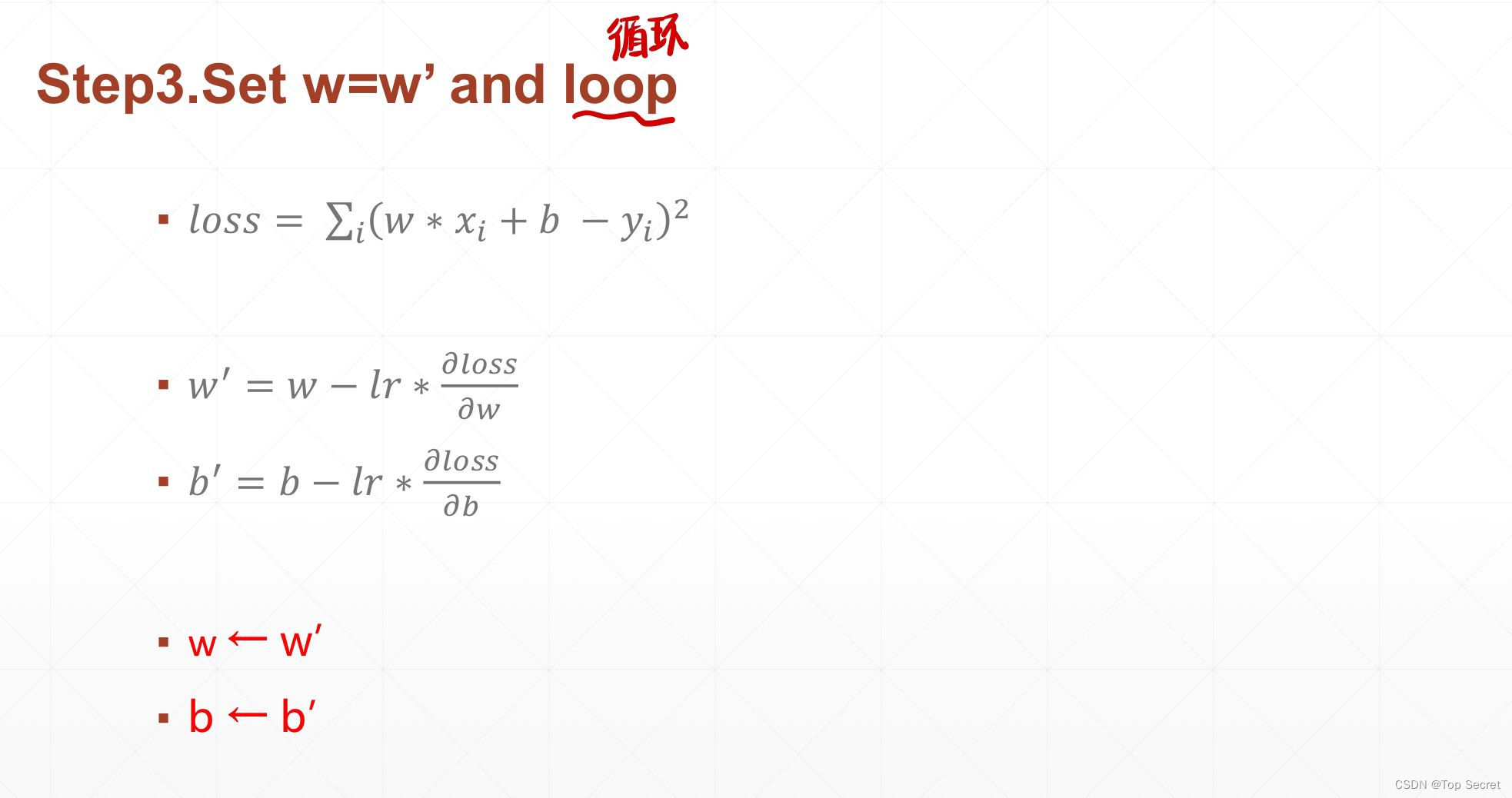
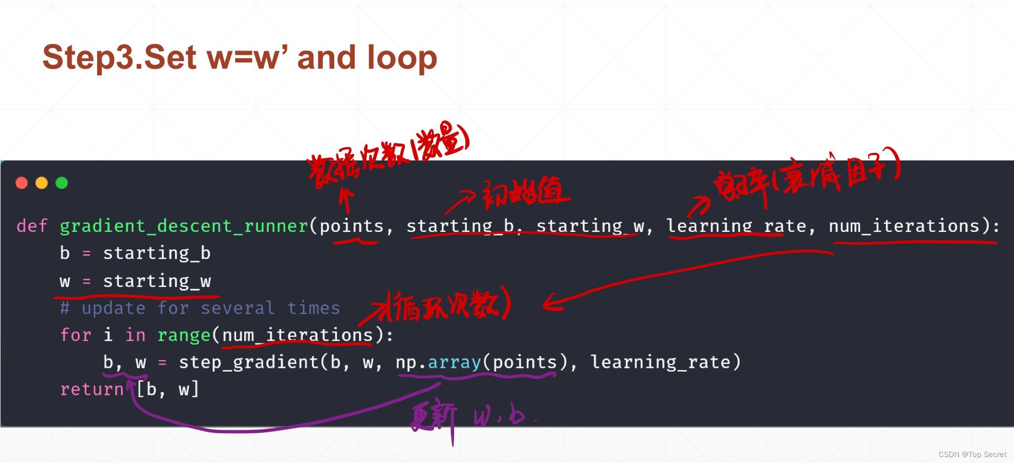
#更新权值w
def gradient_descent_runner(points, starting_b, starting_w, learning_rate, num_iterations):
    b = starting_b
    w = starting_w
    # update for several times
    for i in range(num_iterations):
        b, w = step_gradient(b, w, np.array(points), learning_rate)
    return [b, w]

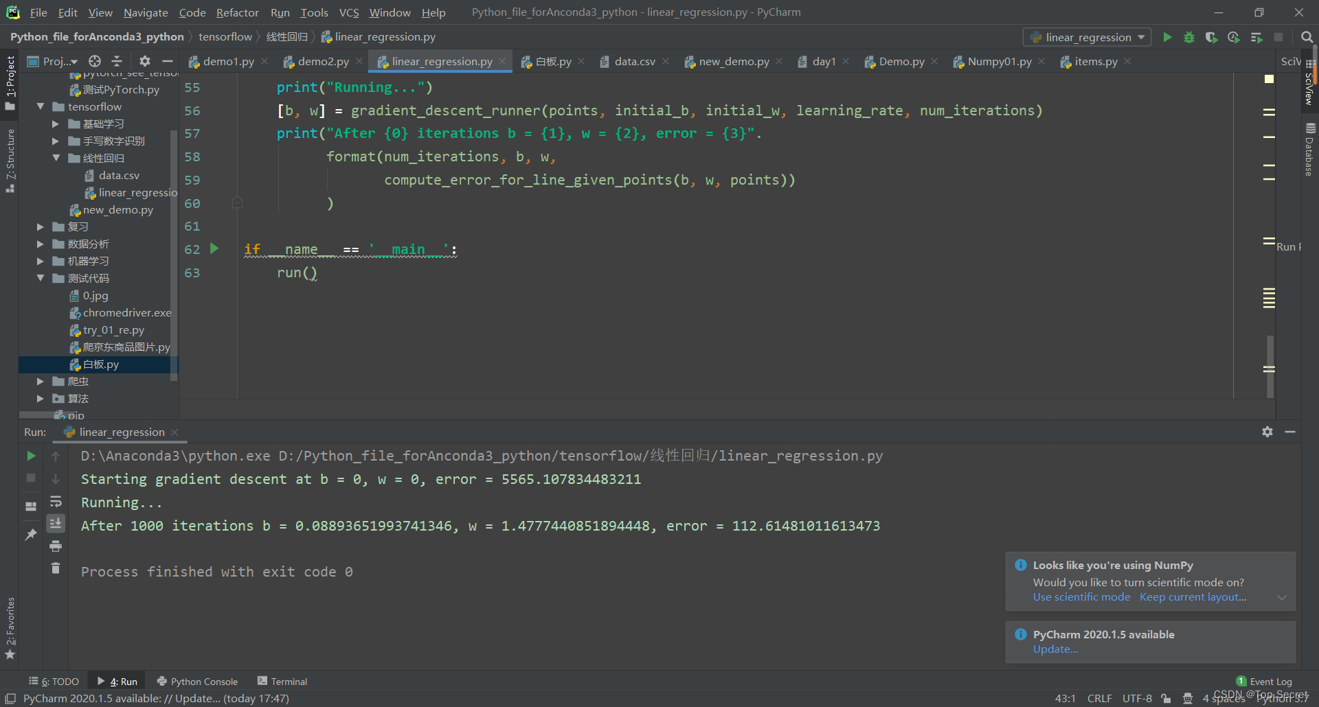
step4:主函数

def run():
    
    points = np.genfromtxt("data.csv", delimiter=",")   #读取数据
    learning_rate = 0.0001  #学习率
    initial_b = 0 # initial y-intercept guess
    initial_w = 0 # initial slope guess
    num_iterations = 1000 
    print("Starting gradient descent at b = {0}, w = {1}, error = {2}"
          .format(initial_b, initial_w,
                  compute_error_for_line_given_points(initial_b, initial_w, points))
          )
    print("Running...")
    [b, w] = gradient_descent_runner(points, initial_b, initial_w, learning_rate, num_iterations)
    print("After {0} iterations b = {1}, w = {2}, error = {3}".
          format(num_iterations, b, w,
                 compute_error_for_line_given_points(b, w, points))
          )

if __name__ == '__main__':
    run()

2.1.1 线性回归问题的全部代码：

import numpy as np

# 实现一个线性回归的问题
# y = wx + b
# step1: 计算损失函数loss的值
def compute_error_for_line_given_points(b, w, points):  #points表示数据的数量
    totalError = 0   #初始化损失函数的值
    for i in range(0, len(points)):
        x = points[i, 0]
        y = points[i, 1]
        # computer mean-squared-error
        totalError += (y - (w * x + b)) ** 2   #求loss的累积和
    # average loss for each point
    return totalError / float(len(points))

# step2:计算梯度与更新
def step_gradient(b_current, w_current, points, learningRate):
    b_gradient = 0
    w_gradient = 0
    N = float(len(points))
    for i in range(0, len(points)):
        x = points[i, 0]
        y = points[i, 1]
        # grad_b = 2(wx+b-y)
        b_gradient += (2/N) * ((w_current * x + b_current) - y)
        # grad_w = 2(wx+b-y)*x
        w_gradient += (2/N) * x * ((w_current * x + b_current) - y)
    # update w'
    new_b = b_current - (learningRate * b_gradient)
    new_w = w_current - (learningRate * w_gradient)
    return [new_b, new_w]

#更新权值w
def gradient_descent_runner(points, starting_b, starting_w, learning_rate, num_iterations):
    b = starting_b
    w = starting_w
    # update for several times
    for i in range(num_iterations):
        b, w = step_gradient(b, w, np.array(points), learning_rate)
    return [b, w]

def run():
    
    points = np.genfromtxt("data.csv", delimiter=",")   #读取数据
    learning_rate = 0.0001  #学习率
    initial_b = 0 # initial y-intercept guess
    initial_w = 0 # initial slope guess
    num_iterations = 1000
    print("Starting gradient descent at b = {0}, w = {1}, error = {2}"
          .format(initial_b, initial_w,
                  compute_error_for_line_given_points(initial_b, initial_w, points))
          )
    print("Running...")
    [b, w] = gradient_descent_runner(points, initial_b, initial_w, learning_rate, num_iterations)
    print("After {0} iterations b = {1}, w = {2}, error = {3}".
          format(num_iterations, b, w,
                 compute_error_for_line_given_points(b, w, points))
          )

if __name__ == '__main__':
    run()

​

2. torch实现线性回归模型

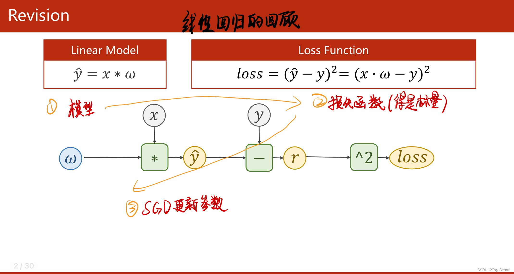
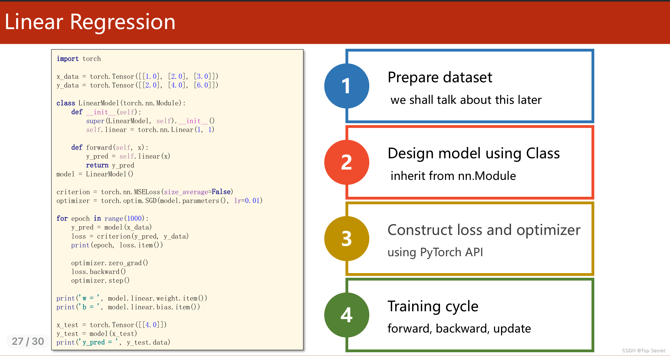
2.1 pytorch构建神经网络的基本步骤

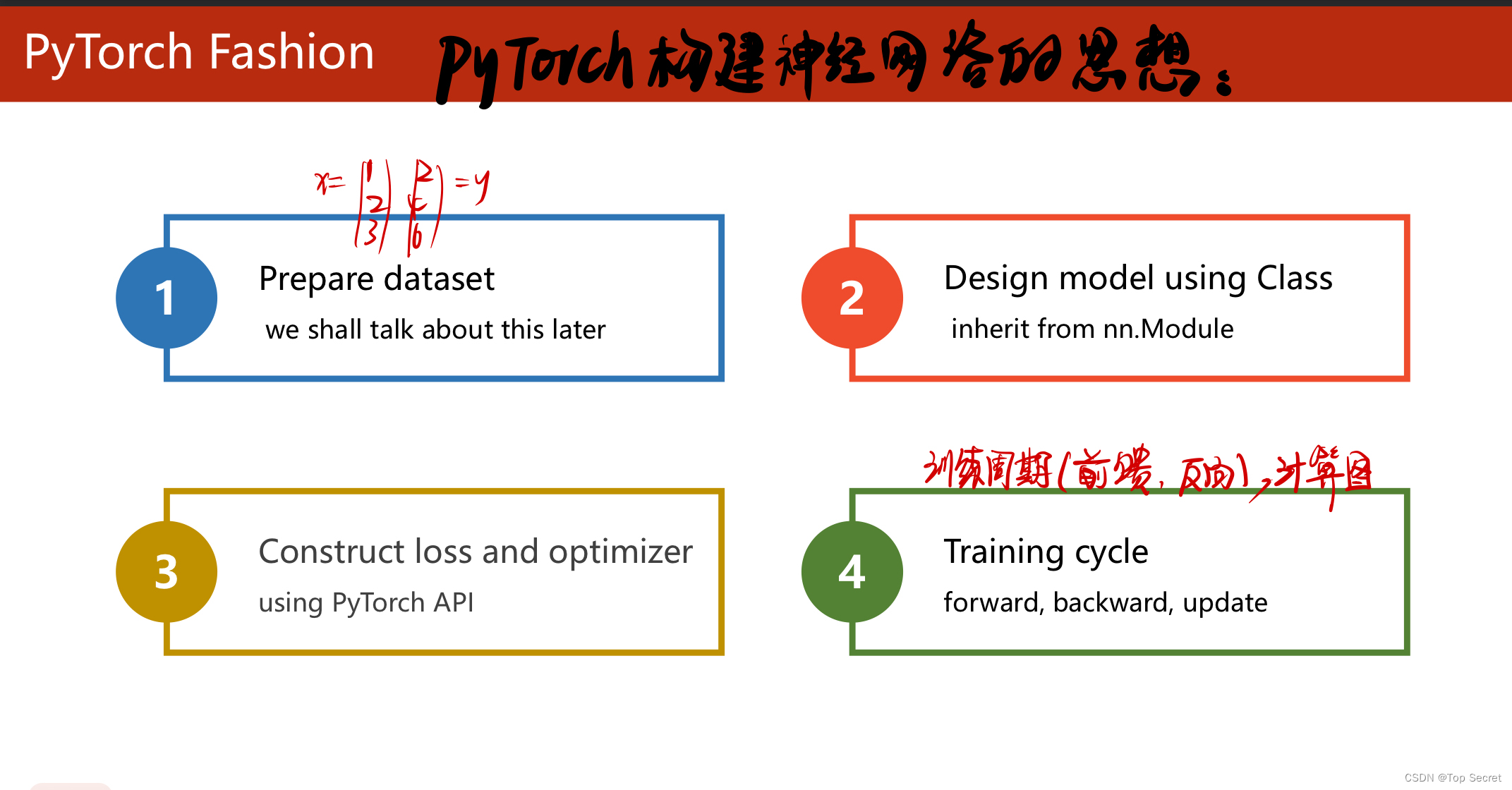
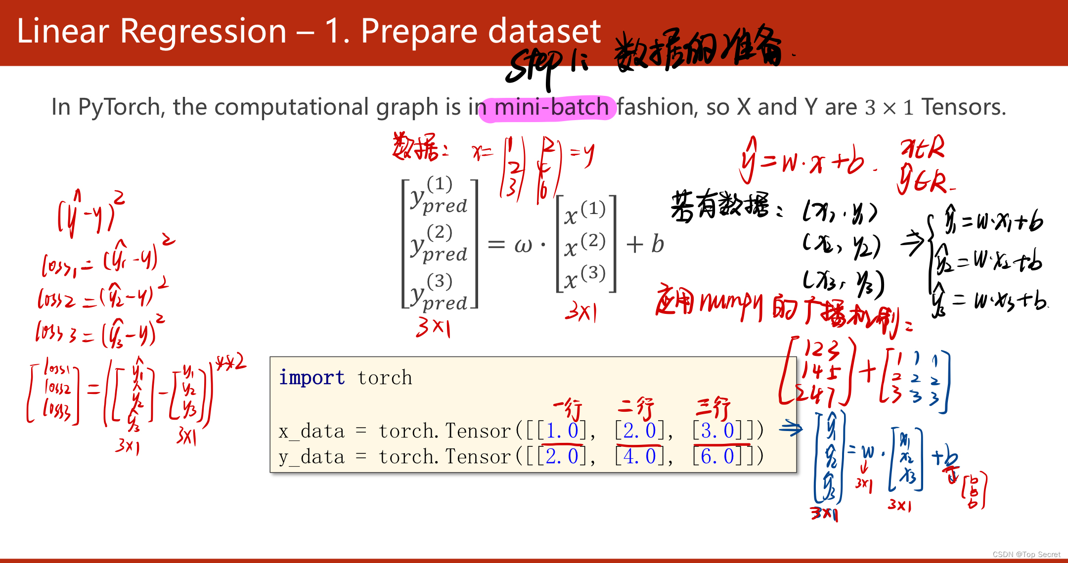
step1:数据集的准备

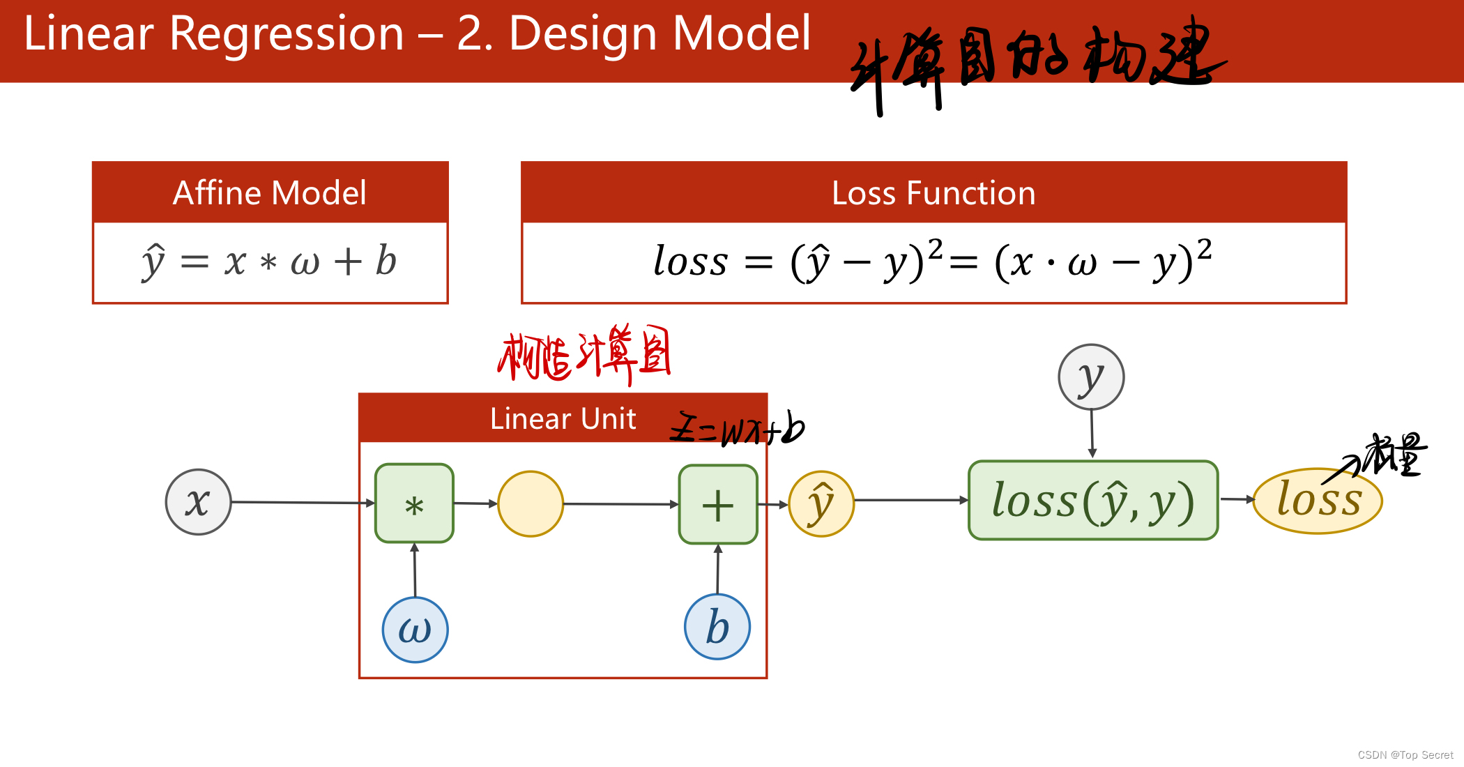
step2:构建数学模型

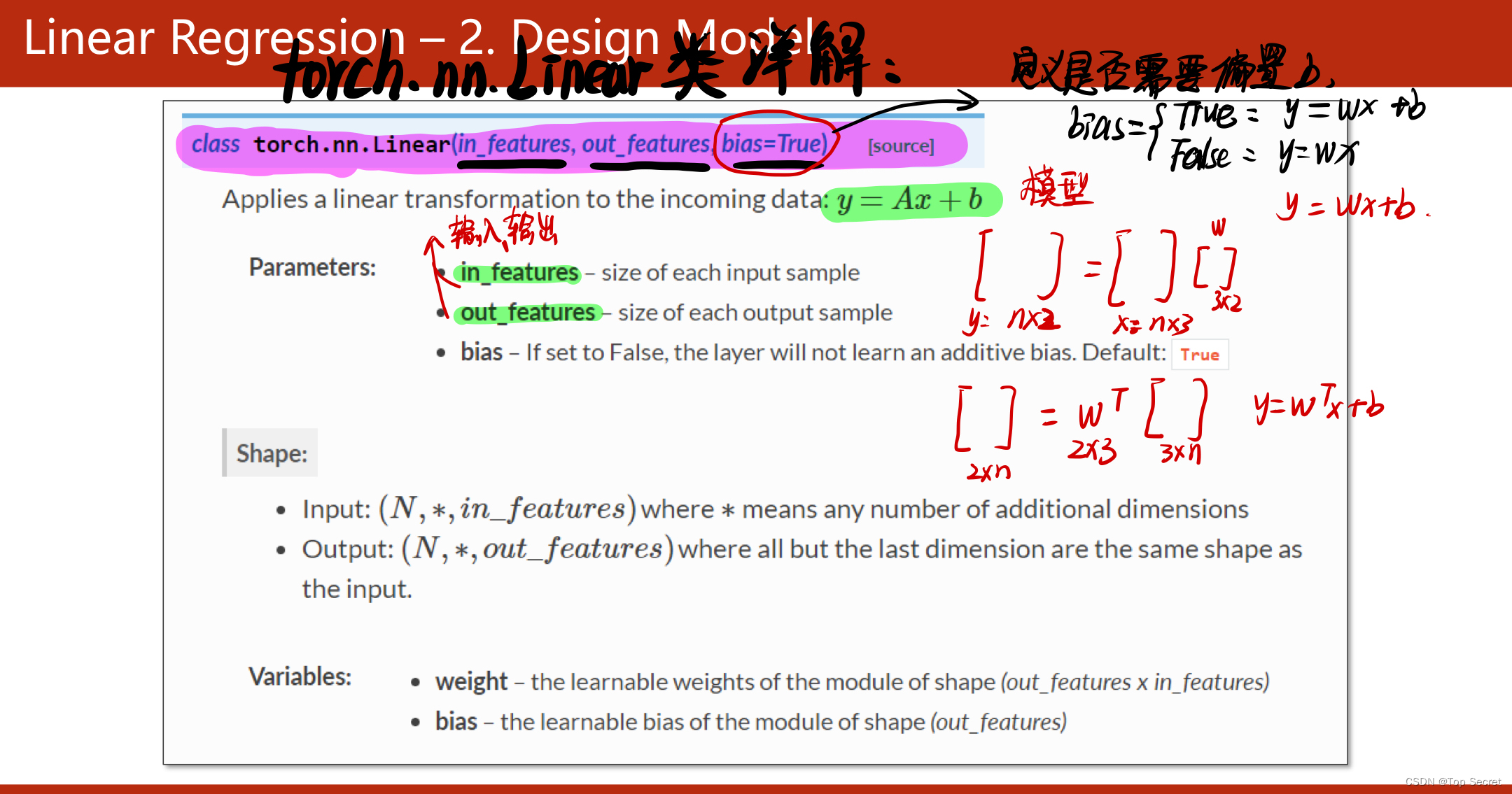
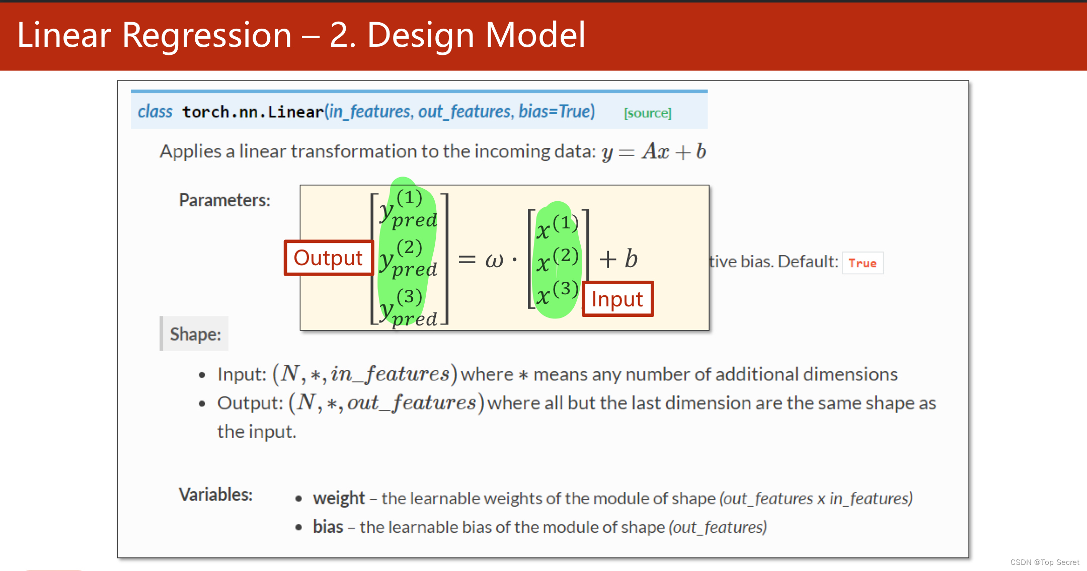
torch.nn.Linear类

step3:构造损失函数与优化器

作业：

step4:训练模型

step5:训练测试集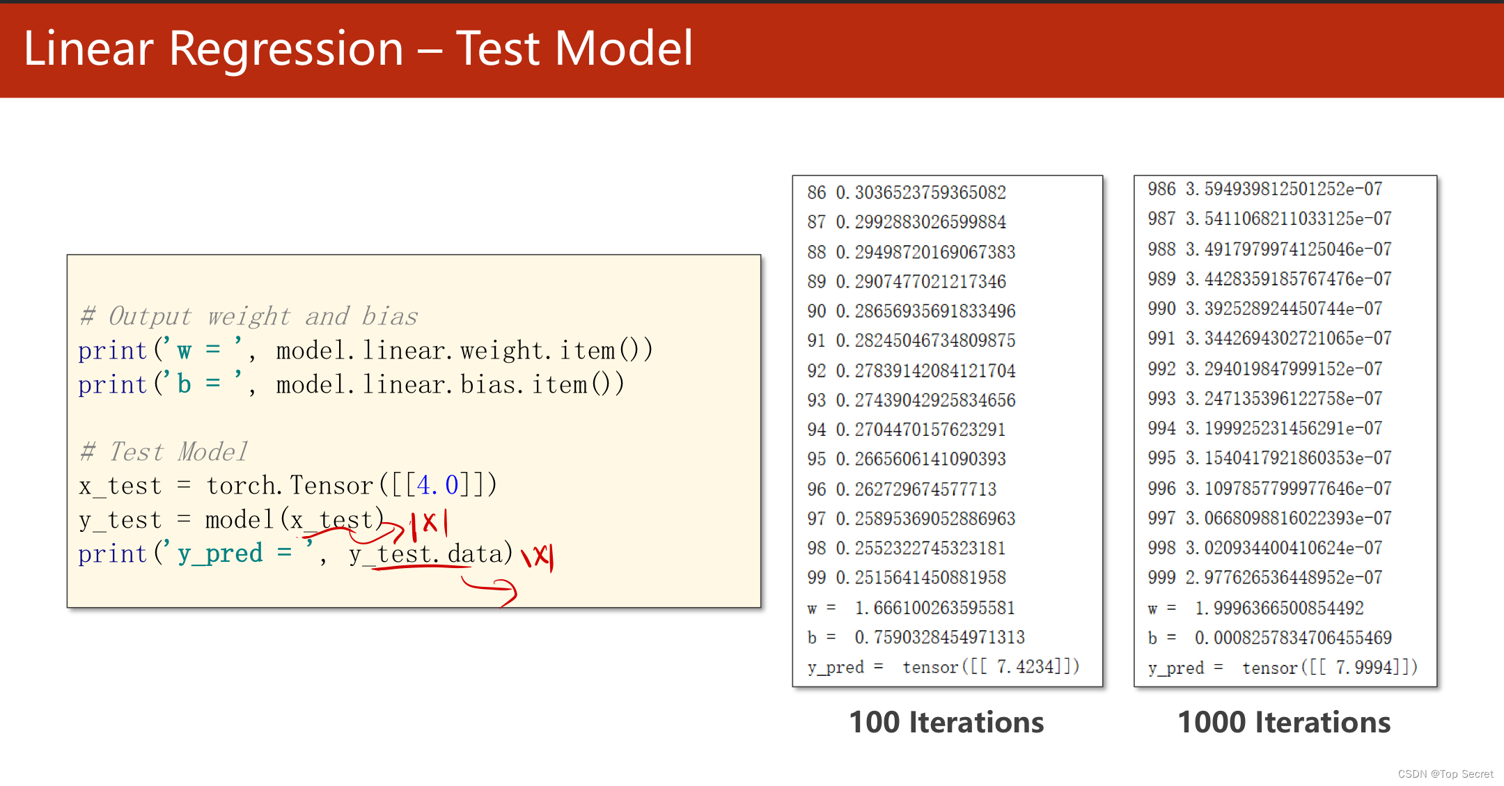

网址：Learning PyTorch with Examples — PyTorch Tutorials 1.12.1+cu102 documentation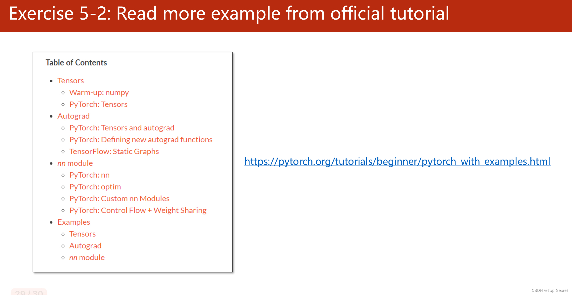

2.2 pytorch代码

实现前后，可以对比一下此文中的内容：
PyTorch 深度学习实践 第5讲_错错莫的博客-CSDN博客

import torch

#step1：prepare dataset
x_data = torch.Tensor([[1.0],[2.0],[3.0]]) #一共三行数据
y_data = torch.Tensor([[2.0],[4.0],[6.0]])

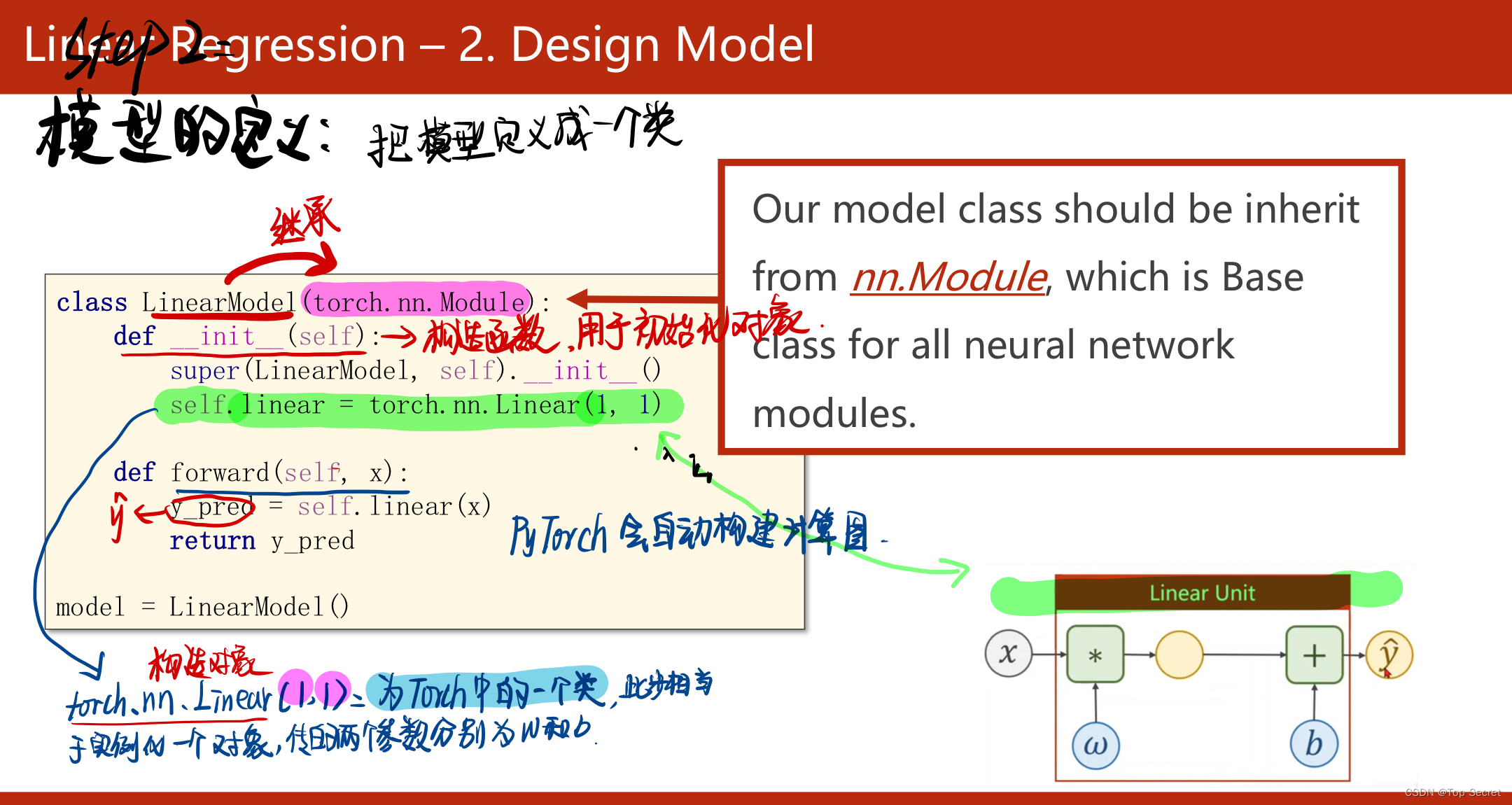
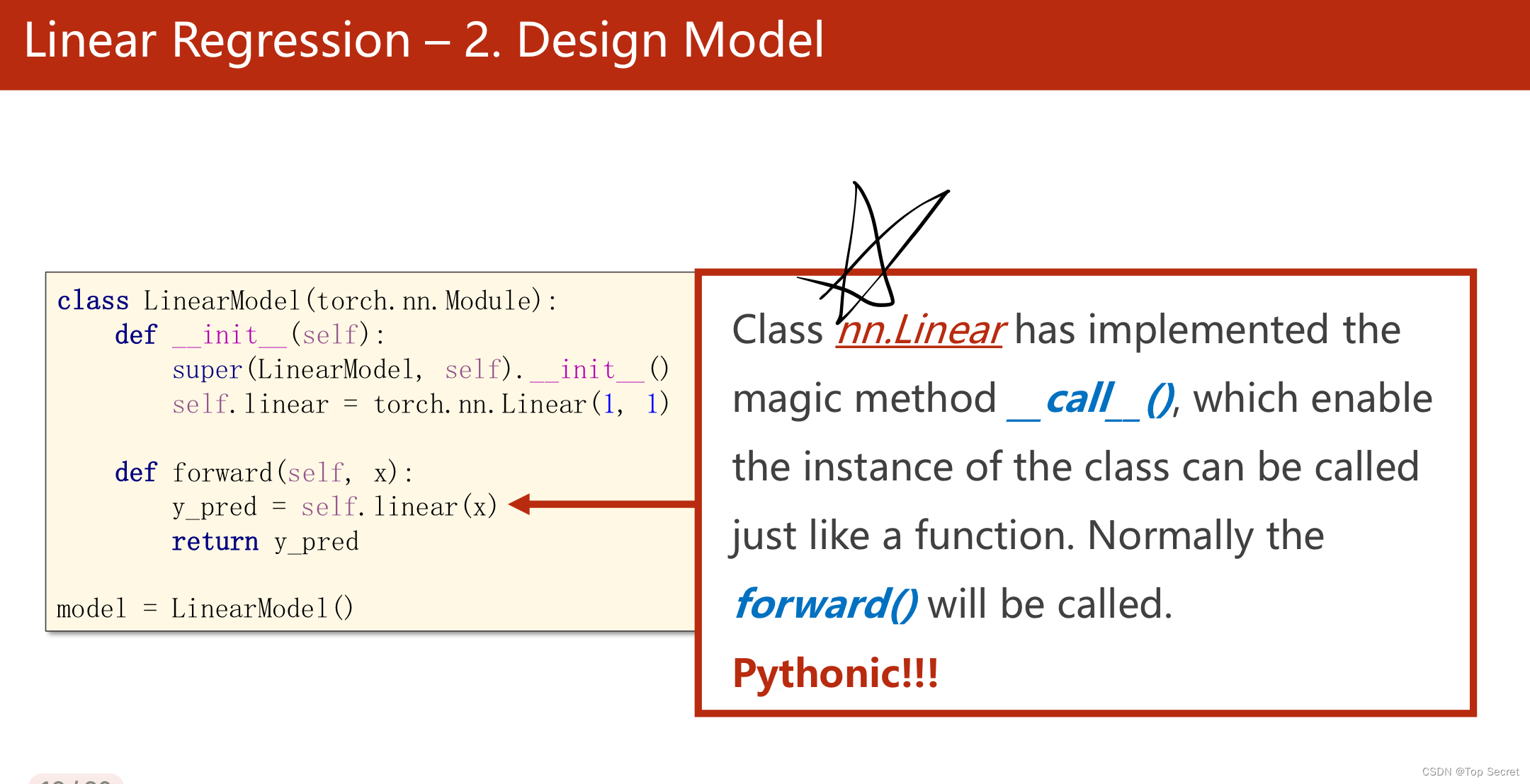
#step2：定义模型(以线性模型为例)
class LinearModel(torch.nn.Module): #构建自己的数学模型需要继承torch的torch.nn.Module类
    def __init__(self):  #构造函数，用于初始化对象
        super(LinearModel, self).__init__()
        # torch.nn.Linear() 也是torch的一个类，此处相当于实例化一个对象，传入的参数为权重w和偏置b
        self.linear = torch.nn.Linear(1,1)

        #该函数即数学模型的直接实现，返回求得的预测值
    def forward(self,x):
        y_pred = self.linear(x)
        return y_pred

model = LinearModel()

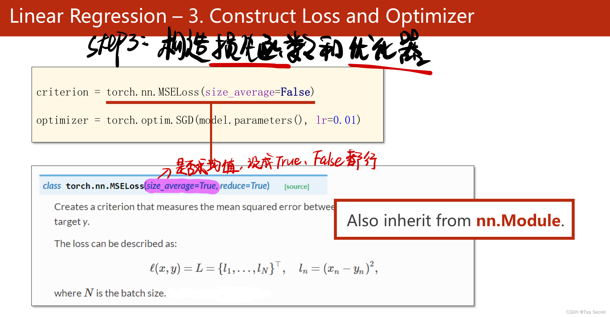
#step3:构造损失函数和优化器
criterion = torch.nn.MSELoss(size_average=False) #选用均方差损失
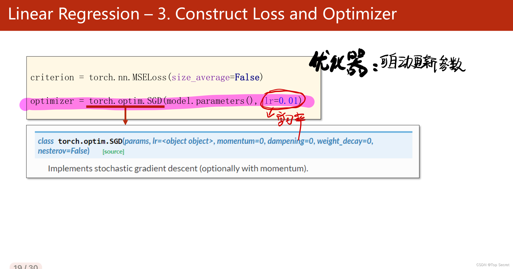
optimizer = torch.optim.SGD(model.parameters(),lr=0.01) # 优化器，用于自动更新参数

if __name__ == '__main__':
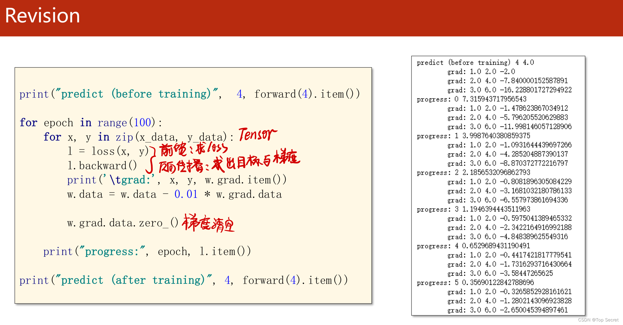
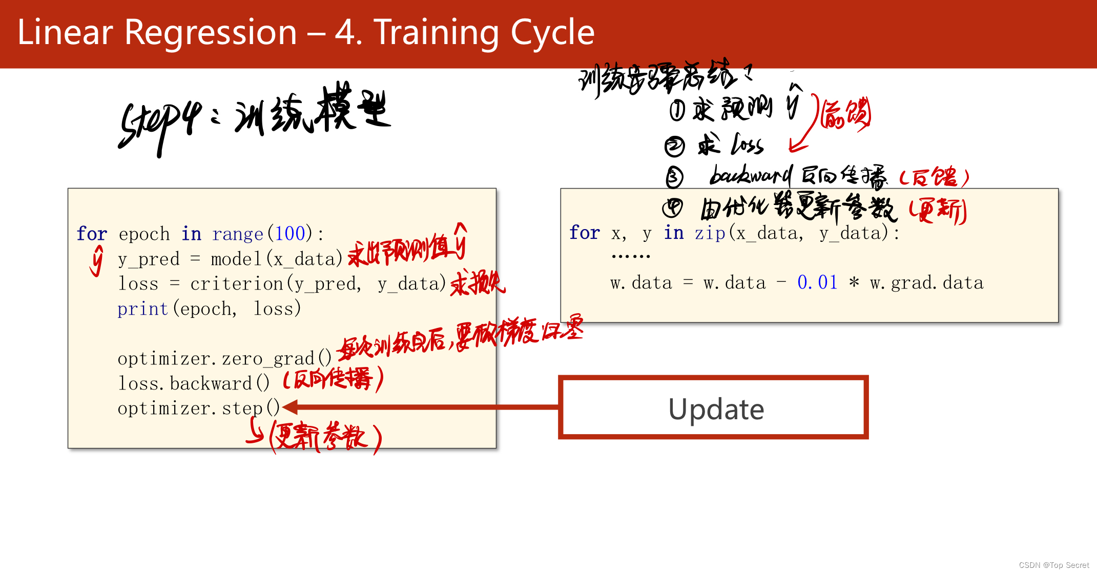
    #step4:训练模型
    for epoch in range(100): #将所有数据训练100次
        y_pred = model(x_data) #求得预测值
        loss = criterion(y_pred,y_data) #求损失函数
        print("当前训练epoch为:",epoch,"损失函数loss值为：",loss)

        optimizer.zero_grad() #梯度清理
        loss.backward() #反向传播
        optimizer.step() #更新参数

    #打印更新的权值w和偏置b
    print('w =',model.linear.weight.item())
    print('b =', model.linear.bias.item())

    #训练测试集
    x_test = torch.Tensor([[4.0]])
    y_test = model(x_test)
    print('y_pred = ',y_test.data)

结果：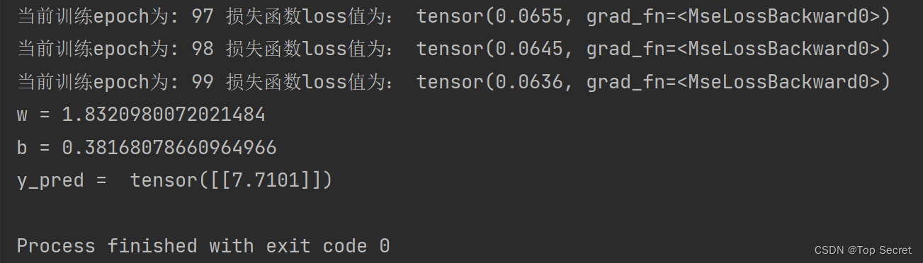

2.3 代码2（和1其实一样，注释不一样而已）

import torch

# prepare dataset
# x,y是矩阵，3行1列 也就是说总共有3个数据，每个数据只有1个特征
x_data = torch.tensor([[1.0], [2.0], [3.0]])
y_data = torch.tensor([[2.0], [4.0], [6.0]])

# design model using class
"""
our model class should be inherit from nn.Module, which is base class for all neural network modules.
member methods __init__() and forward() have to be implemented
class nn.linear contain two member Tensors: weight and bias
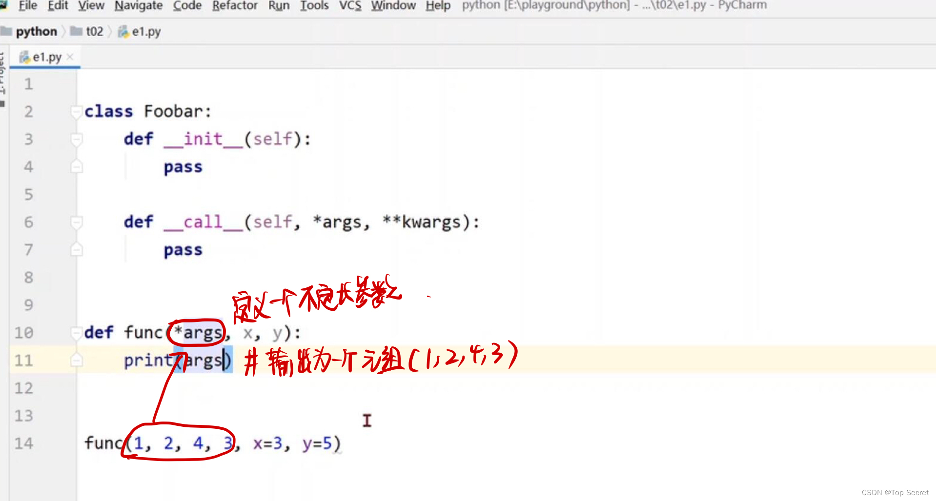
class nn.Linear has implemented the magic method __call__(),which enable the instance of the class can
be called just like a function.Normally the forward() will be called 
"""

class LinearModel(torch.nn.Module):
    def __init__(self):
        super(LinearModel, self).__init__()
        # (1,1)是指输入x和输出y的特征维度，这里数据集中的x和y的特征都是1维的
        # 该线性层需要学习的参数是w和b  获取w/b的方式分别是~linear.weight/linear.bias
        self.linear = torch.nn.Linear(1, 1)

    def forward(self, x):
        y_pred = self.linear(x)
        return y_pred

model = LinearModel()

# construct loss and optimizer
# criterion = torch.nn.MSELoss(size_average = False)
criterion = torch.nn.MSELoss(reduction='sum')
optimizer = torch.optim.SGD(model.parameters(), lr=0.01)  # model.parameters()自动完成参数的初始化操作

# training cycle forward, backward, update
for epoch in range(100):
    y_pred = model(x_data)  # forward:predict
    loss = criterion(y_pred, y_data)  # forward: loss
    print(epoch, loss.item())

    optimizer.zero_grad()  # the grad computer by .backward() will be accumulated. so before backward, remember set the grad to zero
    loss.backward()  # backward: autograd，自动计算梯度
    optimizer.step()  # update 参数，即更新w和b的值

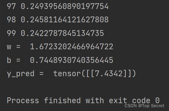
print('w = ', model.linear.weight.item())
print('b = ', model.linear.bias.item())

x_test = torch.tensor([[4.0]])
y_test = model(x_test)
print('y_pred = ', y_test.data)

结果：