
AdaBoost 是集成学习中的一个常见的算法,它模仿“群体智慧”的原理:将单独表现不佳的模型组合起来可以形成一个强大的模型。
麻省理工学院(MIT) 2021年发表的一项研究[Diz21]描述了人们如何识别假新闻。如果没有背景知识或事实的核查,人们往往很难识别假新闻。但是根据不同人的经验,通常可以给出一个对于新闻真假程度的个人见解,这通常比随机猜测要好。如果我们想知道一个标题是描述了真相还是假新闻只需随机询问100个人。如果超过50人说是假新闻,我们就把它归类为假新闻。
将多个弱学习者的预测组合起来,就形成了一个强学习者,它能够准确地分辨真伪,通过集成学习,我们模仿了这个概念
Boosting 是最流行的集成学习技术之一。通过建立了一组所谓的弱学习器,即性能略好于随机猜测的模型。将单个弱学习器的输出组合为加权和,代表分类器的最终输出。AdaBoost是Adaptive Boosting的缩写。自适应Adaptive 是因为一个接一个的建立模型,前一个模型的性能会影响后一个模型的建立过程。
在学习过程中,AdaBoost 算法还会为每个弱学习器分配一个权重,并非每个弱学习器对集成模型的预测都有相同的影响。这种计算整体模型预测的过程称为软投票,类似的如果每个弱学习器的结果权重相等,我们称之为说硬投票。
与Bagging(随机森林)不同,在 Bagging 中,训练的是一组相互独立的单独模型。各个模型彼此不同,因为它们是使用训练数据集的不同随机子集进行训练。随机森林就是基于这个原理,一组单独的决策树形成了集成模型的预测。
而Boosting 的训练是连续的,单个模型的模型构建过程一个接一个地进行,模型预测的准确性会影响后续模型的训练过程。本文将逐步解释 AdaBoost 算法究竟是如何做到这一点的。这些模型由弱学习器、深度为 1 的简单决策树(即所谓的“decision stumps”,我们将其翻译为决策树桩)表示,本文将。
为了更方便得逐步解释 AdaBoost 算法背后的概念,我们选择了一个常见的并且简单得数据集:成年人收入的数据集(“Adult” dataset)。
这个数据集也被称为“人口普查收入”数据集,是一个用于二元分类任务得数据集。该数据集包含描述生活在美国的人们的数据,包括性别、年龄、婚姻状况和教育等属性。目标变量区分低于和高于每年 50,000 美元的收入。
为了说明 AdaBoost 算法的工作原理,我简化了数据集,并且只使用了其中的一小部分。在本文的最后提供代码的下载。
首先载入数据集
import pandas as pd

 df=pd.read_csv("<https://archive.ics.uci.edu/ml/machine-learning-databases/adult/adult.data>",
                  names= ["age",
                             "workclass",
                             "fnlwgt",
                             "education",
                             "education-num",
                             "marital-status",
                             "occupation",
                             "relationship",
                             "race",
                             "sex",
                             "capital-gain",
                             "capital-loss",
                             "hours-per-week",
                             "native-country",
                             "income"],
                  index_col=False)
为了详细解释算法是如何工作的,我们这里只使用 3 个简单的二进制特征:
- 性别:男(是或否)
- 每周工作时间:>40 小时(是或否)
- 年龄:>50 (是或否)
 importnumpyasnp

 # define input parameter
 df['male'] =df['sex'].apply(lambdax : 'Yes'ifx.lstrip() =="Male"else"No")
 df['>40 hours'] =np.where(df['hours-per-week']>40, 'Yes', 'No')
 df['>50 years'] =np.where(df['age']>50, 'Yes', 'No')

 # target
 df['>50k income'] =df['income'].apply(lambdax : 'Yes'ifx.lstrip() =='>50K'else"No")

 # define dataset
 df_simpl=df[['male', '>40 hours','>50 years','>50k income']]
 df_simpl=df_simpl.head(10)
 df_simpl
下面我就用这个简单的数据集来解释AdaBoost算法的工作原理。
1、构建第一个弱学习者:找到性能最好的“树桩”
第一步,我们需要寻找一个弱学习者,它可以对我们的目标(>50k 收入)进行简单得规则判断,并且要比随机猜测要好。
AdaBoost 可以与多种机器学习算法结合使用。一般情况下我们会选择决策树作为弱学习者,这是 AdaBoost 算法最流行的方式:
决策树在所谓的节点处逐步拆分整个数据集。树中的第一个节点称为根节点,所有节点都在决策节点之后。不再对数据集进行拆分的节点称为终端节点或叶节点。
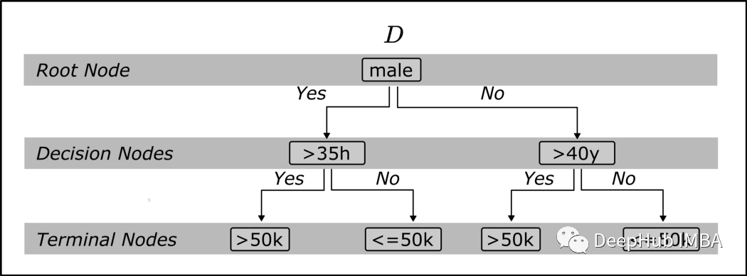
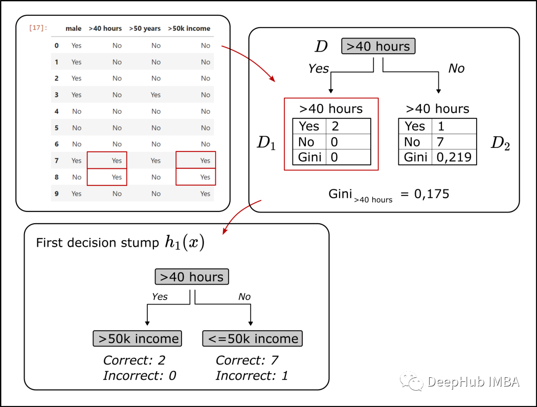
为了构建出最佳性能的第一个决策树桩。我们构建能够确定数据集中最有可能区分收入高于和低于 50k 的决策树模型。
我们从一个随机选择的特征开始;这里的示例特征是“男性”。这个属性只能区分一个人是不是男人。根节点将整个数据集分割为一个子集,其中只有男性和所有其他类型的实例。
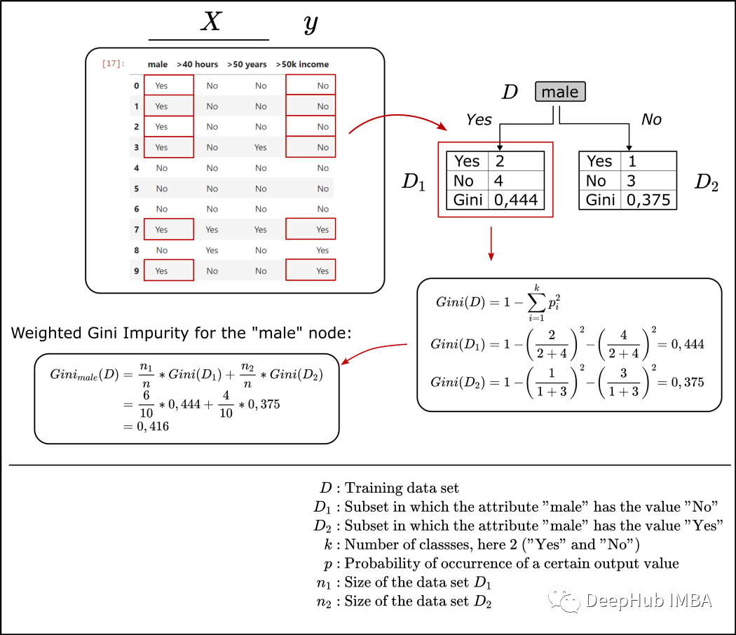
如果一个子集(例如D_1)包含k个不同的类,那么一条记录属于类i的概率可以描述为p_i。在下面的图片中,我描述了如何计算左侧末节的基尼不纯度。
我们演示的简单数据集只包含10个实例:6个为男性,4个为女性。如果我们观察6个“男性”数据样本的子集D_1,会发现6个样本中有4个的收入是50k或以下,只有2个记录收入在5万以上。子集D_1的随机样本显示收入高于50k的概率是2/6或1/3,样本显示收入低于50k的概率是4/6或2/3。因此叶子1(子集D_1)的基尼系数不纯度为0.444。
如果我们对叶子2做同样的操作,我们得到不纯度为0.375。
由于我们要比较根节点“男性”、“>40 小时”和“>50 年”的树桩的性能/基尼指数,我们首先计算根节点“男性”的加权 不纯度作为加权单个叶子的总和。
下面的Python代码片段中实现了基尼系数的计算,它只是简单地遍历数据帧的所有列,并执行上面描述的基尼系数计算:
 defcalc_weighted_gini_index(attribute, df):
     '''
     Args:
         df: the trainings dataset stored in a data frame
         attribute: the chosen attribute for the root node of the tree
     Return:
         Gini_attribute: the gini index for the chosen attribute
     '''

     d_node=df[[attribute, '>50k income']]

     # number of records in the dataset (=10, for the simple example)
     n=len(d_node)

     # number of values "Yes" and "No" for the target variable ">50k income" in the root node
     n_1=len(d_node[d_node[attribute] =='Yes'])
     n_2=len(d_node[d_node[attribute] =='No'])

     # count "Yes" and "No" values for the target variable ">50k income" in each leafe
     # left leafe, D_1
     n_1_yes=len(d_node[(d_node[attribute] =='Yes') & (d_node[">50k income"] =='Yes')])
     n_1_no=len(d_node[(d_node[attribute] =='Yes') & (d_node[">50k income"] =='No')])

     # right leafe, D_2
     n_2_yes=len(d_node[(d_node[attribute] =='No') & (d_node[">50k income"] =='Yes')])
     n_2_no=len(d_node[(d_node[attribute] =='No') & (d_node[">50k income"] =='No')])

     # Gini index of the left leafe
     Gini_1=1-(n_1_yes/(n_1_yes+n_1_no)) **2-(n_1_no/(n_1_yes+n_1_no)) **2

     # Gini index of the right leafe
     Gini_2=1-(n_2_yes/(n_2_yes+n_2_no)) **2-(n_2_no/(n_2_yes+n_2_no)) **2

     # weighted Gini index for the selected feature (=attribute) as root node
     Gini_attribute= (n_1/n) *Gini_1+ (n_2/n) *Gini_2
     Gini_attribute=round(Gini_attribute, 3)

     print(f'Gini_{attribute} = {Gini_attribute}')

     returnGini_attribute

 deffind_attribute_that_shows_the_smallest_gini_index(df):
     '''
     Args:
         df: the trainings dataset stored in a data frame
     Return:
         selected_root_node_attribute: the attribute/feature that showed the lowest gini index
     '''

     # calculate gini index for each attribute in the dataset and store them in a list
     attributes= []
     gini_indexes= []

     forattributeindf.columns[:-1]:
         # calculate gini index for attribute as root note using the defined function "calc_weighted_gini_index"
         gini_index=calc_weighted_gini_index(attribute, df)

         attributes.append(attribute)
         gini_indexes.append(gini_index)

     # create a data frame using the just calculated gini index for each feature/attribute of the dataset
     print("Calculated Gini indexes for each attribute of the data set:")

     d_calculated_indexes= {'attribute':attributes,'gini_index':gini_indexes}
     d_indexes_df=pd.DataFrame(d_calculated_indexes)

     display(d_indexes_df)

     # Find the attribute for the first stump, the attribute where the Gini index is lowest the thus the Gini gain is highest")
     selected_root_node_attribute=d_indexes_df.min()["attribute"]

     print(f"Attribute for the root node of the stump: {selected_root_node_attribute}")

     returnselected_root_node_attribute

 ################################################################################################################
 # to build the first stump we are using the orginial dataset as the train dataset
 # the defined functions identify the features with the highest Gini gain
 ################################################################################################################
 df_step_1=df_simpl
 selected_root_node_attribute=find_attribute_that_shows_the_smallest_gini_index(df_step_1)
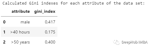
我们的目标是最小化叶子的基尼不纯度,从而最大化基尼增益,基尼增益是通过两个分割子集的加权不纯度与整个数据集的不纯度之差来计算的。
通过计算我们发现工作时间特征为“>40小时”的基尼增益最高,所以我们使用它建立了第一个“树桩”。
AdaBoost 现在会按顺序构建“树桩”,但是 AdaBoost 的特性(也是一个问题)是:第一个“树桩”的错误会影响下一个“树桩”的建模过程。错误分类的实例在下一棵树中的权重更大,单个“树桩”的结果在集成模型中的加权程度取决于误差有多高。
2、计算“树桩”的误差
在上图中已经绘制了正确和错误分类实例的数量:在预测目标变量时,构建的第一个“树桩”只有一个错误(数据集中只有一个实例是每周工作时间超过 40 小时但年收入低于 5 万)。数据集中的所有其他实例已经用这个简单的决策“树桩”正确分类。
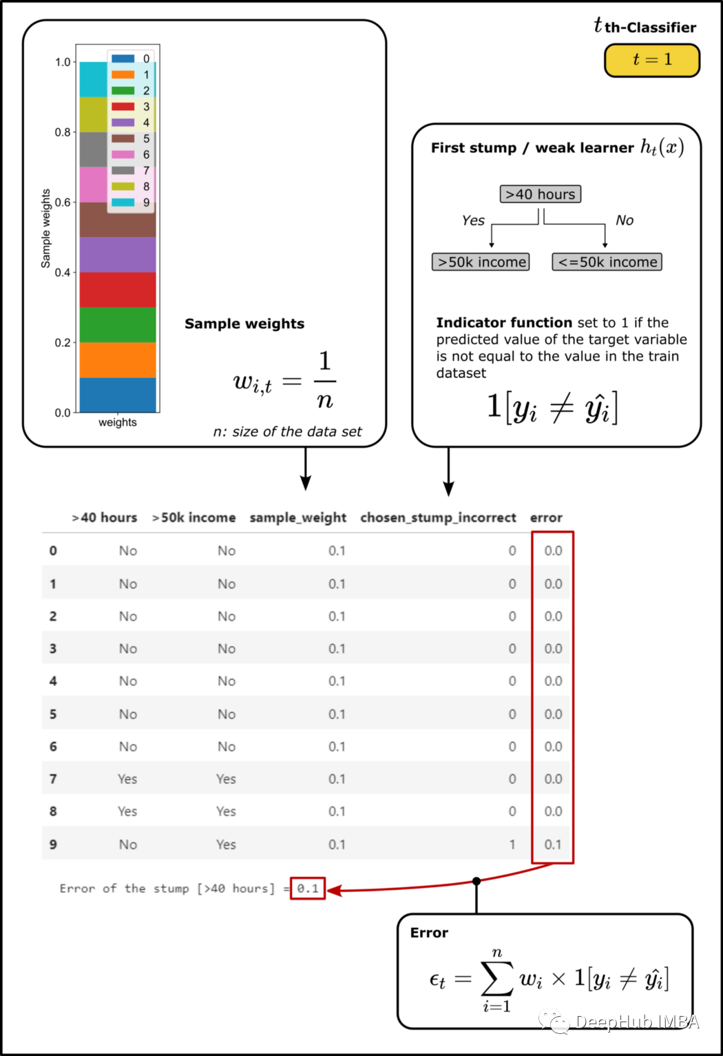
为了计算误差值需要为数据集的每条记录引入权重。在第一个“树桩”形成之前,每个实例的权重 w 为 w=1/n,其中 n 对应于数据集的总数据大小,所有权重的总和为 1。
决策树桩产生的误差被简单地计算为“树桩”错误分类目标变量的所有样本权重的总和。这里错误分类只有一个,所以第一次运行的误差为 1/10。
下面的函数“calculate_error_for_chosen_stump”用选择的特征作为根节点(selected_root_node_attribute)计算加权误差。
 importhelper_functions
 defcalculate_error_for_chosen_stump(df, selected_root_node_attribute):
     '''
     Attributes:
         df: trainings data set
         selected_root_node_attribute: name of the column used for the root node of the stump

     Return:
         df_extended: df extended by the calculated weights and error
         error: calculated error for the stump - sum of the weights of all samples that were misclassified by the decision stub
     '''
     # add column for the sample weight, for the first step its simply defined as 1/n, so the sum of all weights is 1
     df["sample_weight"] =1/len(df)
     df[selected_root_node_attribute]
     df[">50k income"]

     # in binary classification, we have two ways to build the tree.
     # (1) That attribute and target value show the same value or
     # (2) attribute and target value show the opposite value
     # we choose the one which shows less errors
     # stump_1_incorrect_v1 and stump_1_incorrect_v2 shows the prediction result of the two stumps
     df["stump_1_incorrect_v1"] =np.where(((df[selected_root_node_attribute] =="Yes") & (df[">50k income"] =="Yes")) |
                                              ((df[selected_root_node_attribute] =="No") & (df[">50k income"] =="No")),0,1)
     df["stump_1_incorrect_v2"] =np.where(((df[selected_root_node_attribute] =="Yes") & (df[">50k income"] =="No")) |
                                              ((df[selected_root_node_attribute] =="No") & (df[">50k income"] =="Yes")),0,1)

     # select the stump with fewer samples misclassified
     ifsum(df['stump_1_incorrect_v1']) <=sum(df["stump_1_incorrect_v2"]):
         df["chosen_stump_incorrect"] =df['stump_1_incorrect_v1']
     else:
         df["chosen_stump_incorrect"] =df['stump_1_incorrect_v2']

     # drop the columns for the two versions of the tree
     df=df.drop(['stump_1_incorrect_v1', 'stump_1_incorrect_v2'], axis=1)

     # calculate the error by multiplying sample weight and the column chosen_stump_incorrect
     df["error"] =df["sample_weight"] *df["chosen_stump_incorrect"]
     error=sum(df["error"])

     # data frame extended by the weights, errors, etc.
     df_extended=df

     # display extended dataset
     display(df_extended[[selected_root_node_attribute,">50k income","sample_weight", "chosen_stump_incorrect", "error"]])

     # plot calculated weights in a stacked bar-plot
     helper_functions.plot_weights(df_extended)

     print(f'Error of the stump [{selected_root_node_attribute}] = {error}')
     returndf_extended, error

 # call function to calculate the weighted error for the selected stump
 df_extended_1, error=calculate_error_for_chosen_stump(df_step_1, selected_root_node_attribute)
3、计算“树桩”的权重,也就是“发言权”
集成模型的结果是所有“树桩”预测的加权和。所以下面我们要确认刚刚构建的树的预测对于最终集成模型的重要性。或者换句话说,权重alpha有多高。
我们计算alpha的数量如下:
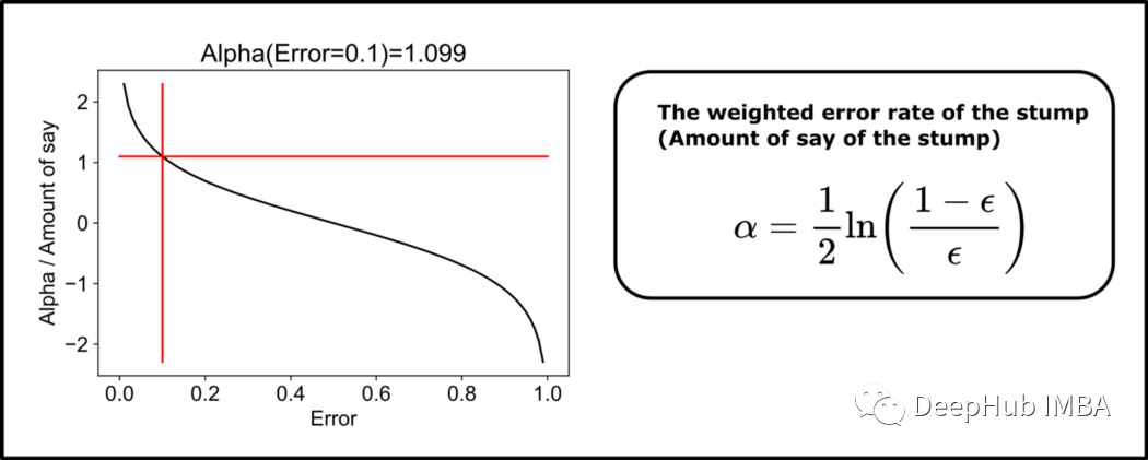
上图左侧显示了alpha与“树桩”加权误差之间的关系。对于小错误,alpha量很大。对于较大的错误,alpha 甚至可以取负值。对于第一个树桩的误差为 0.1,所以最后计算的发言权重约为 1.1。
 importmatplotlib.pyplotasplt
 fromdatetimeimportdatetime

 # calculate the amount of say using the weighted error rate of the weak classifier
 alpha=1/2*np.log((1-error)/error)
 print(f'Amount of say / Alpha = {round(alpha,3)}')

 helper_functions.plot_alpha(alpha, error)
4、调整样本权重
由于我们在建模第二个“树桩“时要考虑第一个的结果,所以我们根据第一个的误差来调整样本权值。第一个预测错误的数据集的记录应该在构建下一个树桩的过程中发挥更大的作用,所以首先调整各个样本的权重。
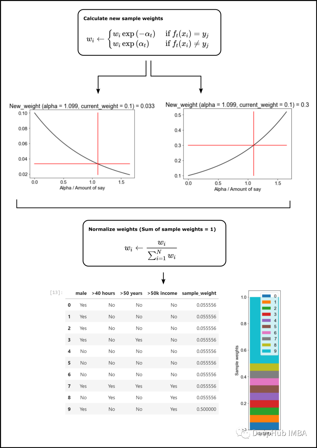
新权重用alpha计算如下:
左图显示了正确分类样本的比例,右边的图表显示了错误分类样本的比例,对新的样本权值进行归一化处理
下面代码计算和绘制新的权重比例:
 importmath


 defplot_scale_of_weights(alpha, current_sample_weight, incorrect):
     alpha_list= []
     new_weights= []

     ifincorrect==1:
         # adjust the sample weights for instances which were misclassified
         new_weight=current_sample_weight*math.exp(alpha)

         # calculate x and y for plot of the scaling function and new sample weight
         foralpha_ninnp.linspace(0, alpha*1.5, num=100):
             scale=current_sample_weight*math.exp(alpha_n)
             alpha_list.append(alpha_n)
             new_weights.append(scale)
     else:
         # adjust the sample weights for instances which were classified correct
         new_weight=current_sample_weight*math.exp(-alpha)

         # calculate x and y for plot of the scaling function and new sample weight
         foralpha_ninnp.linspace(0, alpha*1.5, num=100):
             scale=current_sample_weight*math.exp(-alpha_n)
             alpha_list.append(alpha_n)
             new_weights.append(scale)

     ######################################################################################################
     # plot scaling of the sample weight
     ######################################################################################################
     # change font size for matplotlib graph
     font= {'family': 'arial',
             'weight': 'normal',
             'size': 15}
     plt.rc('font', **font)

     plt.plot(alpha_list, new_weights, color='black')
     plt.plot(np.linspace(alpha, alpha, num=100), new_weights, color='red')
     plt.plot(np.linspace(0, alpha*1.5, num=100), np.linspace(new_weight, new_weight, num=100), color='red')

     plt.xlabel('Alpha / Amount of say')
     plt.title(
         f'New_weight (alpha = {round(alpha, 3)}, current_weight = {round(current_sample_weight, 3)}) = {round(new_weight, 3)}')

     # define plot name and save the figure
     # datetime object containing current date and time
     now=datetime.now()

     # use timestamp for file name
     # dd/mm/YY H:M:S
     dt_string=now.strftime("%d_%m_%Y_%H_%M_%S")
     plt.savefig(r'.\\plots\\sample_weights_'+dt_string+'.svg')

     plt.show()

     returnnew_weight


 new_weight=plot_scale_of_weights(alpha, current_sample_weight=0.1, incorrect=1)
使用上面定义的函数来更新样本权重:
 defupdate_sample_weights(df_extended_1):
     # calculate the new weights for the misclassified samples
     defcalc_new_sample_weight(x, alpha):
         new_weight=plot_scale_of_weights(alpha, x["sample_weight"], x["chosen_stump_incorrect"])
         returnnew_weight
     df_extended_1["new_sample_weight"] =df_extended_1.apply(lambdax: calc_new_sample_weight(x, alpha), axis=1)

     # define new extended data frame
     df_extended_2=df_extended_1[["male", ">40 hours", ">50 years", ">50k income", "new_sample_weight"]]
     df_extended_2=df_extended_2.rename(columns={"new_sample_weight": "sample_weight"}, errors="raise")

     # normalize weights
     df_extended_2["sample_weight"] =df_extended_2["sample_weight"] *1/df_extended_2["sample_weight"].sum()
     df_extended_2["sample_weight"].sum()
     returndf_extended_2

 df_extended_2=update_sample_weights(df_extended_1)
5、第二次运行:形成一个新的自举数据集
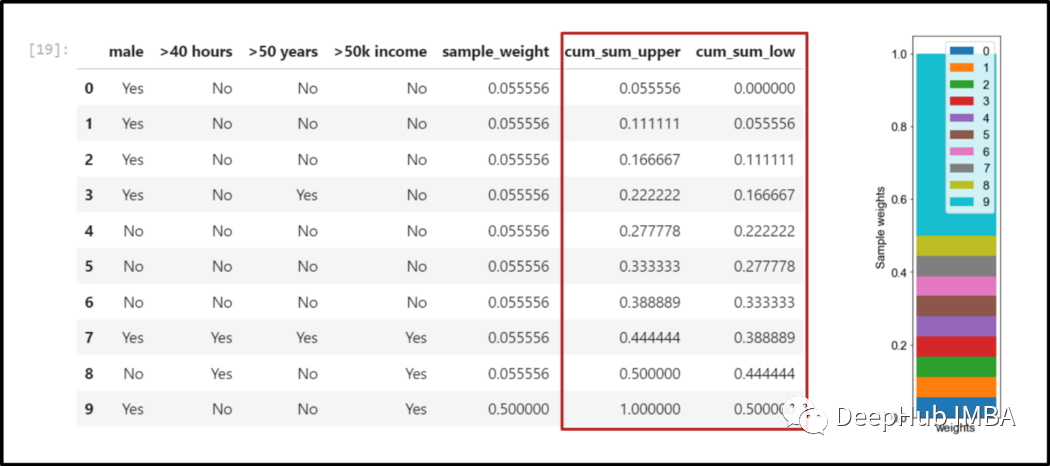
第二次运行还是简单地为每个属性建立一个”树桩"并选择加权误差最小的,但是这不是一个好办法,所以我们使用样本权重来生成一个新的数据集,其中权重更大的样本会被认为在统计上更常见。我使用样本权重将范围0-1分成若干个bins。
在下面图片中看到被描述为“cum_sum_low”-“cum_sum_upper”的bins的范围。
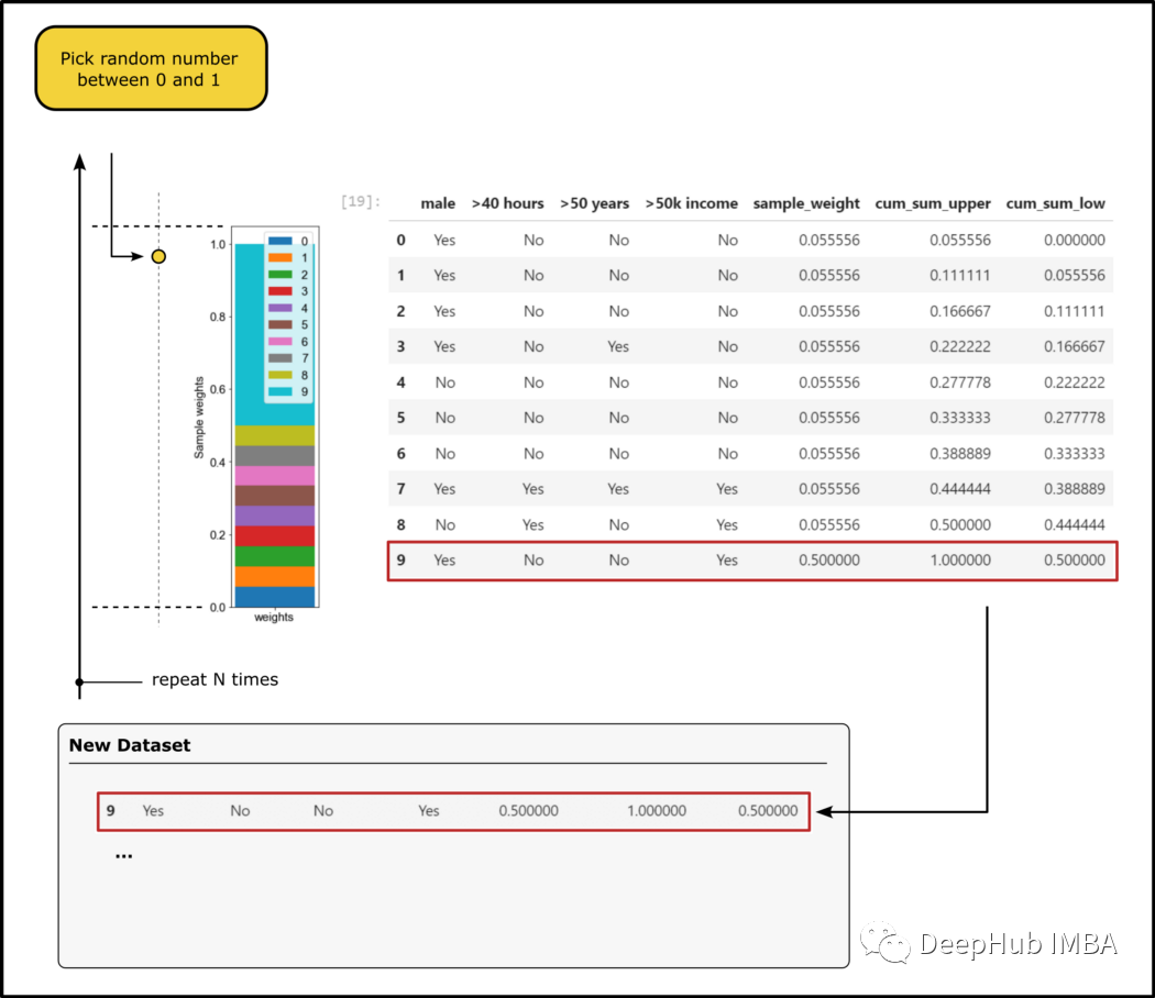
然后选择一个介于 0 和 1 之间的随机数,并查找该数字所属的范围的bin,并将样本添加到新数据集中。重复这个过程 N 次,直到我有一个与原始数据集一大小的新数据集。
由于权重更大的样本在 0 到 1 的范围内会有更大的概率出现,因此权重更大的样本通常在新数据集中出现不止一次。在下图中可以看到:第一个错误分类的样本权重更大(此处权重为 0.5),最终在新数据集中出现的频率更高。
使用新数据集,我们继续重复第一步的工作:
- 计算所有特征的基尼系数,选择特征作为第二个“树桩”的根节点
- 建造第二个树桩
- 将加权误差计算为误分类样本的样本权重之和
 ####################################################################################
 # define bins to select new instances
 ####################################################################################

 importrandom
 df_extended_2["cum_sum_upper"] =df_extended_2["sample_weight"].cumsum()
 df_extended_2["cum_sum_low"] = [0] +df_extended_2["cum_sum_upper"][0:9].to_list()

 ####################################################################################
 # create new dataset
 ####################################################################################
 new_data_set= []
 foriinrange(0,len(df_extended_2),1):
     random_number=random.randint(0, 100)*0.01

     ifi==0:
         picked_instance=df_extended_2[(df_extended_2["cum_sum_low"]<random_number) & (df_extended_2["cum_sum_upper"]>random_number)]
         new_data_set=picked_instance
     else:
         picked_instance=df_extended_2[(df_extended_2["cum_sum_low"]<random_number) & (df_extended_2["cum_sum_upper"]>random_number)]
         new_data_set=pd.concat([new_data_set, picked_instance], ignore_index=True)

 new_data_set
找到第二个""树桩""的根节点:
 df_step_2=new_data_set[["male", ">50 years", ">50k income"]]
 selected_root_node_attribute_2=find_attribute_that_shows_the_smallest_gini_index(df_step_2)
6、重复这个过程,直到达到终止条件
算法会重复我们上面描述的1-5步,直到达到某个终止条件,例如直到所有特征都被用作根节点一次。所有的步骤总结如下:
- 找到最大化基尼收益的弱学习器 h_t(x)(或者最小化错误分类实例的误差)
- 将弱学习器的加权误差计算为错误分类样本的样本权重之和。
- 将分类器添加到集成模型中。模型的结果是对各个弱学习器结果的总结。使用上面确定的“发言权重”/加权错误率 (alpha) 对弱学习者进行加权。
- 更新发言权重:在加权和误差的帮助下,将 alpha 计算为刚刚形成的弱学习器的“发言权重”。
- 使用这个 alpha 来重新调整样本权重。
- 新的样本权重被归一化,使权重之和为 1
- 使用新的权重,通过在 0 和 1 之间选择一个随机数 N 次来生成一个新的数据集,然后将数据样本添加到表示该数据集的新数据集中。
- 通过新数据集训练新的弱学习器(与步骤1相同)
7、将弱学习器组合成一个集成模型
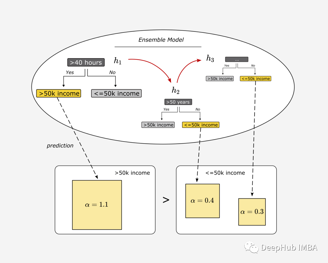
到目前为止,我们只差一个将弱学习器进行组合的过程没有说明了,这个过程很简单,就是对每个“树桩”进行预测。
对于这个简单的例子,一个 30 岁的人每周工作 42 小时,第一个预测的结果是收入高于 50k,第二个结果是收入低于 50k。
我们将收入超过 5 万的结果和收入低于 5 万的结果的权重相加。
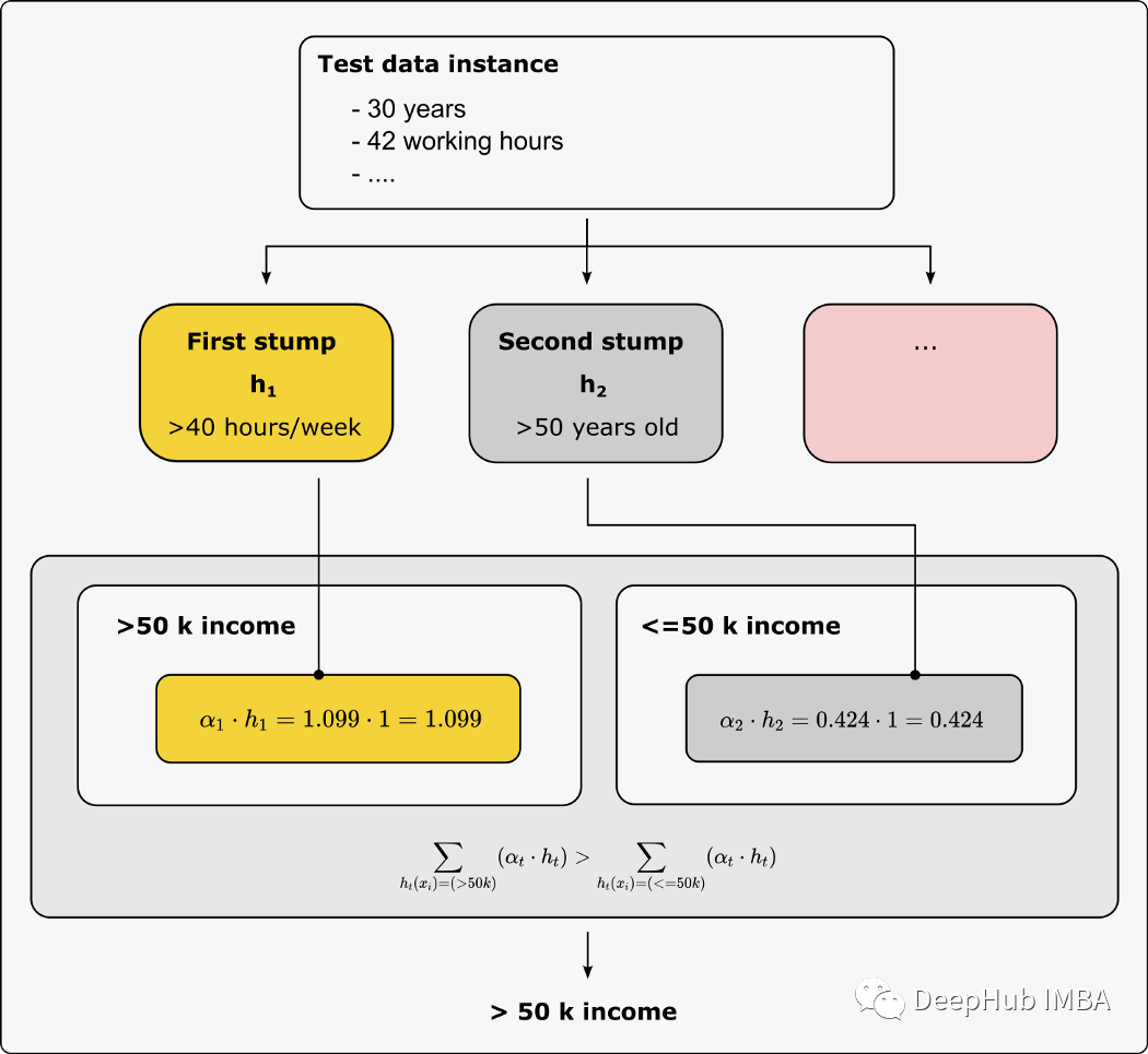
然后比较权重的总和。在我们的例子中,第一个"树桩"的权重占主导地位,因此集成模型的预测是收入 >50k,代码如下:
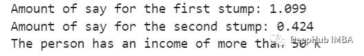
 alpha_step_1=alpha
 print(f"Amount of say for the first stump: {round(alpha_step_1,3)}")

 alpha_step_2=alpha_step_2
 print(f"Amount of say for the second stump: {round(alpha_step_2,3)}")
 ##########################################################################################
 # Make a prediction:
 # Suppose a person lives in the U.S., is 30 years old, and works about 42 hours per week.
 ##########################################################################################
 # the first stump uses the hours worked per week (>40 hours) as the root node
 # if the regular working hours per week is above 40 hours, the stump would say that the person earns more than 50 k
 # otherwise, the income would be classified as below 50 k
 F_1=1
 # the second stump uses the age (>50 years) as root node
 # if you are over 50 years old, you are more likely to have an income of more than 50 k
 # in this case, our second weak learner would classifier the target variable (>50 k income) as a 'Yes' or 1
 # otherwise as a 'No' or 0
 F_2=0
 # calculate the result of the ensemble model
 F_over_50_k=alpha_step_1*1+alpha_step_2*0
 F_below_50_k=alpha_step_1*0+alpha_step_2*1
 ifF_over_50_k>F_below_50_k:
     print("The person has an income of more than 50 k")
 else:
     print("The person has an income below 50 k")
总结
Boosting 方法在近年来的多项数据竞赛中都取得了优异的成绩,但其背后的概念却并不复杂。通过使用简单易懂的步骤构建简单并且可解释的模型,然后将简单模型的组合成强大的学习器。
本文代码:
https://github.com/polzerdo55862/Ada-Boost-Tutorial
本文参考:
[Diz21] Peter Dizikes: MIT News, 2021. https://news.mit.edu/2021/crowd-source-fact-checking-0901
[Kar22] Fatih Karabiber: Gini Impurity, 2022. https://www.learndatasci.com/glossary/gini-impurity/
[Kum21] Ajitesh Kumar: Hard vs Soft Voting Classifier Python Example, 2021. https://vitalflux.com/hard-vs-soft-voting-classifier-python-example/
[Koh96] Kohavi, Ronny and Becker, Barry: Adult datas set, 1996. https://archive.ics.uci.edu/ml/datasets/adult (CC BY 4.0)
[Wiq20] Wiqaas: Boosting a decision stump, 2020. https://github.com/wiqaaas/youtube/blob/master/Machine_Learning_from_Scratch/AdaBoosting/AdaBoosting_Decision_Tree.ipynb
作者:Dominik Polzer