
Diffusion扩散模型学习1——Pytorch搭建DDPM利用深度卷积神经网络实现图片生成
学习前言
我又死了我又死了我又死了!
源码下载地址
https://github.com/bubbliiiing/ddpm-pytorch
喜欢的可以点个star噢。
网络构建
一、什么是Diffusion

如上图所示。DDPM模型主要分为两个过程:
1、Forward加噪过程(从右往左),数据集的真实图片中逐步加入高斯噪声,最终变成一个杂乱无章的高斯噪声,这个过程一般发生在训练的时候。加噪过程满足一定的数学规律。
2、Reverse去噪过程(从左往右),指对加了噪声的图片逐步去噪,从而还原出真实图片,这个过程一般发生在预测生成的时候。尽管在这里说的是加了噪声的图片,但实际去预测生成的时候,是随机生成一个高斯噪声来去噪。去噪的时候不断根据
X
t
X_t
Xt的图片生成
X
t
−
1
X_{t-1}
Xt−1的噪声,从而实现图片的还原。
1、加噪过程
Forward加噪过程主要符合如下的公式:
x
t
=
α
t
x
t
−
1
+
1
−
α
t
z
1
x_t=\sqrt{\alpha_t} x_{t-1}+\sqrt{1-\alpha_t} z_{1}
xt=αtxt−1+1−αtz1
其中
α
t
\sqrt{\alpha_t}
αt是预先设定好的超参数,被称为Noise schedule,通常是小于1的值,在论文中
α
t
\alpha_t
αt的值从0.9999到0.998。
ϵ
t
−
1
∼
N
(
0
,
1
)
\epsilon_{t-1} \sim N(0, 1)
ϵt−1∼N(0,1)是高斯噪声。由公式(1)迭代推导。
x
t
=
a
t
(
a
t
−
1
x
t
−
2
+
1
−
α
t
−
1
z
2
)
+
1
−
α
t
z
1
=
a
t
a
t
−
1
x
t
−
2
+
(
a
t
(
1
−
α
t
−
1
)
z
2
+
1
−
α
t
z
1
)
x_t=\sqrt{a_t}\left(\sqrt{a_{t-1}} x_{t-2}+\sqrt{1-\alpha_{t-1}} z_2\right)+\sqrt{1-\alpha_t} z_1=\sqrt{a_t a_{t-1}} x_{t-2}+\left(\sqrt{a_t\left(1-\alpha_{t-1}\right)} z_2+\sqrt{1-\alpha_t} z_1\right)
xt=at(at−1xt−2+1−αt−1z2)+1−αtz1=atat−1xt−2+(at(1−αt−1)z2+1−αtz1)
其中每次加入的噪声都服从高斯分布
z
1
,
z
2
,
…
∼
N
(
0
,
1
)
z_1, z_2, \ldots \sim \mathcal{N}(0, 1)
z1,z2,…∼N(0,1),两个高斯分布的相加高斯分布满足公式:
N
(
0
,
σ
1
2
)
+
N
(
0
,
σ
2
2
)
∼
N
(
0
,
(
σ
1
2
+
σ
2
2
)
)
\mathcal{N}\left(0, \sigma_1^2 \right)+\mathcal{N}\left(0, \sigma_2^2 \right) \sim \mathcal{N}\left(0,\left(\sigma_1^2+\sigma_2^2\right) \right)
N(0,σ12)+N(0,σ22)∼N(0,(σ12+σ22)),因此,得到
x
t
x_t
xt的公式为:
x
t
=
a
t
a
t
−
1
x
t
−
2
+
1
−
α
t
α
t
−
1
z
2
x_t = \sqrt{a_t a_{t-1}} x_{t-2}+\sqrt{1-\alpha_t \alpha_{t-1}} z_2
xt=atat−1xt−2+1−αtαt−1z2
因此不断往里面套,就能发现规律了,其实就是累乘
可以直接得出
x
0
x_0
x0到
x
t
x_t
xt的公式:
x
t
=
α
t
‾
x
0
+
1
−
α
t
‾
z
t
x_t=\sqrt{\overline{\alpha_t}} x_0+\sqrt{1-\overline{\alpha_t}} z_t
xt=αtx0+1−αtzt
其中
α
t
‾
=
∏
i
t
α
i
\overline{\alpha_t}=\prod_i^t \alpha_i
αt=∏itαi,这是随Noise schedule设定好的超参数,
z
t
−
1
∼
N
(
0
,
1
)
z_{t-1} \sim N(0, 1)
zt−1∼N(0,1)也是一个高斯噪声。通过上述两个公式,我们可以不断的将图片进行破坏加噪。
2、去噪过程
反向过程就是通过估测噪声,多次迭代逐渐将被破坏的
x
t
x_t
xt恢复成
x
0
x_0
x0,在恢复时刻,我们已经知道的是
x
t
x_t
xt,这是图片在
t
t
t时刻的噪声图。一下子从
x
t
x_t
xt恢复成
x
0
x_0
x0是不可能的,我们只能一步一步的往前推,首先从
x
t
x_t
xt恢复成
x
t
−
1
x_{t-1}
xt−1。根据贝叶斯公式,已知
x
t
x_t
xt反推
x
t
−
1
x_{t-1}
xt−1:
q
(
x
t
−
1
∣
x
t
,
x
0
)
=
q
(
x
t
∣
x
t
−
1
,
x
0
)
q
(
x
t
−
1
∣
x
0
)
q
(
x
t
∣
x
0
)
q\left(x_{t-1} \mid x_t, x_0\right)=q\left(x_t \mid x_{t-1}, x_0\right) \frac{q\left(x_{t-1} \mid x_0\right)}{q\left(x_t \mid x_0\right)}
q(xt−1∣xt,x0)=q(xt∣xt−1,x0)q(xt∣x0)q(xt−1∣x0)
右边的三个东西都可以从x_0开始推得到:
q
(
x
t
−
1
∣
x
0
)
=
a
ˉ
t
−
1
x
0
+
1
−
a
ˉ
t
−
1
z
∼
N
(
a
ˉ
t
−
1
x
0
,
1
−
a
ˉ
t
−
1
)
q\left(x_{t-1} \mid x_0\right)=\sqrt{\bar{a}_{t-1}} x_0+\sqrt{1-\bar{a}_{t-1}} z \sim \mathcal{N}\left(\sqrt{\bar{a}_{t-1}} x_0, 1-\bar{a}_{t-1}\right)
q(xt−1∣x0)=aˉt−1x0+1−aˉt−1z∼N(aˉt−1x0,1−aˉt−1)
q
(
x
t
∣
x
0
)
=
a
ˉ
t
x
0
+
1
−
α
ˉ
t
z
∼
N
(
a
ˉ
t
x
0
,
1
−
α
ˉ
t
)
q\left(x_t \mid x_0\right) = \sqrt{\bar{a}_t} x_0+\sqrt{1-\bar{\alpha}_t} z \sim \mathcal{N}\left(\sqrt{\bar{a}_t} x_0 , 1-\bar{\alpha}_t\right)
q(xt∣x0)=aˉtx0+1−αˉtz∼N(aˉtx0,1−αˉt)
q
(
x
t
∣
x
t
−
1
,
x
0
)
=
a
t
x
t
−
1
+
1
−
α
t
z
∼
N
(
a
t
x
t
−
1
,
1
−
α
t
)
q\left(x_t \mid x_{t-1}, x_0\right)=\sqrt{a_t} x_{t-1}+\sqrt{1-\alpha_t} z \sim \mathcal{N}\left(\sqrt{a_t} x_{t-1}, 1-\alpha_t\right) \\
q(xt∣xt−1,x0)=atxt−1+1−αtz∼N(atxt−1,1−αt)
因此,由于右边三个东西均满足正态分布,
q
(
x
t
−
1
∣
x
t
,
x
0
)
q\left(x_{t-1} \mid x_t, x_0\right)
q(xt−1∣xt,x0)满足分布如下:
∝
exp
(
−
1
2
(
(
x
t
−
α
t
x
t
−
1
)
2
β
t
+
(
x
t
−
1
−
α
ˉ
t
−
1
x
0
)
2
1
−
α
ˉ
t
−
1
−
(
x
t
−
α
ˉ
t
x
0
)
2
1
−
α
ˉ
t
)
)
\propto \exp \left(-\frac{1}{2}\left(\frac{\left(x_t-\sqrt{\alpha_t} x_{t-1}\right)^2}{\beta_t}+\frac{\left(x_{t-1}-\sqrt{\bar{\alpha}_{t-1}} x_0\right)^2}{1-\bar{\alpha}_{t-1}}-\frac{\left(x_t-\sqrt{\bar{\alpha}_t} x_0\right)^2}{1-\bar{\alpha}_t}\right)\right)
∝exp(−21(βt(xt−αtxt−1)2+1−αˉt−1(xt−1−αˉt−1x0)2−1−αˉt(xt−αˉtx0)2))
把标准正态分布展开后,乘法就相当于加,除法就相当于减,把他们汇总
接下来继续化简,咱们现在要求的是上一时刻的分布
∝
exp
(
−
1
2
(
(
x
t
−
α
t
x
t
−
1
)
2
β
t
+
(
x
t
−
1
−
α
ˉ
t
−
1
x
0
)
2
1
−
α
ˉ
t
−
1
−
(
x
t
−
α
ˉ
t
x
0
)
2
1
−
α
ˉ
t
)
)
=
exp
(
−
1
2
(
x
t
2
−
2
α
t
x
t
x
t
−
1
+
α
t
x
t
−
1
2
β
t
+
x
t
−
1
2
−
2
α
ˉ
t
−
1
x
0
x
t
−
1
+
α
ˉ
t
−
1
x
0
2
1
−
α
ˉ
t
−
1
−
(
x
t
−
α
ˉ
t
x
0
)
2
1
−
α
ˉ
t
)
)
=
exp
(
−
1
2
(
(
α
t
β
t
+
1
1
−
α
ˉ
t
−
1
)
x
t
−
1
2
−
(
2
α
t
β
t
x
t
+
2
α
ˉ
t
−
1
1
−
α
ˉ
t
−
1
x
0
)
x
t
−
1
+
C
(
x
t
,
x
0
)
)
)
\begin{aligned} & \propto \exp \left(-\frac{1}{2}\left(\frac{\left(x_t-\sqrt{\alpha_t} x_{t-1}\right)^2}{\beta_t}+\frac{\left(x_{t-1}-\sqrt{\bar{\alpha}_{t-1}} x_0\right)^2}{1-\bar{\alpha}_{t-1}}-\frac{\left(x_t-\sqrt{\bar{\alpha}_t} x_0\right)^2}{1-\bar{\alpha}_t}\right)\right) \\ & =\exp \left(-\frac{1}{2}\left(\frac{x_t^2-2 \sqrt{\alpha_t} x_t x_{t-1}+\alpha_t x_{t-1}^2}{\beta_t}+\frac{x_{t-1}^2-2 \sqrt{\bar{\alpha}_{t-1}} x_0 x_{t-1}+\bar{\alpha}_{t-1} x_0^2}{1-\bar{\alpha}_{t-1}}-\frac{\left(x_t-\sqrt{\bar{\alpha}_t} x_0\right)^2}{1-\bar{\alpha}_t}\right)\right) \\ & =\exp \left(-\frac{1}{2}\left(\left(\frac{\alpha_t}{\beta_t}+\frac{1}{1-\bar{\alpha}_{t-1}}\right) x_{t-1}^2-\left(\frac{2 \sqrt{\alpha_t}}{\beta_t} x_t+\frac{2 \sqrt{\bar{\alpha}_{t-1}}}{1-\bar{\alpha}_{t-1}} x_0\right) x_{t-1}+C\left(x_t, x_0\right)\right)\right) \end{aligned}
∝exp(−21(βt(xt−αtxt−1)2+1−αˉt−1(xt−1−αˉt−1x0)2−1−αˉt(xt−αˉtx0)2))=exp(−21(βtxt2−2αtxtxt−1+αtxt−12+1−αˉt−1xt−12−2αˉt−1x0xt−1+αˉt−1x02−1−αˉt(xt−αˉtx0)2))=exp(−21((βtαt+1−αˉt−11)xt−12−(βt2αtxt+1−αˉt−12αˉt−1x0)xt−1+C(xt,x0)))
正态分布满足公式,
exp
(
−
(
x
−
μ
)
2
2
σ
2
)
=
exp
(
−
1
2
(
1
σ
2
x
2
−
2
μ
σ
2
x
+
μ
2
σ
2
)
)
\exp \left(-\frac{(x-\mu)^2}{2 \sigma^2}\right)=\exp \left(-\frac{1}{2}\left(\frac{1}{\sigma^2} x^2-\frac{2 \mu}{\sigma^2} x+\frac{\mu^2}{\sigma^2}\right)\right)
exp(−2σ2(x−μ)2)=exp(−21(σ21x2−σ22μx+σ2μ2)),其中
σ
\sigma
σ就是方差,
μ
\mu
μ就是均值,配方后我们就可以获得均值和方差。
此时的均值为:
μ
~
t
(
x
t
,
x
0
)
=
α
t
(
1
−
α
ˉ
t
−
1
)
1
−
α
ˉ
t
x
t
+
α
ˉ
t
−
1
β
t
1
−
α
ˉ
t
x
0
\tilde{\mu}_t\left(x_t, x_0\right)=\frac{\sqrt{\alpha_t}\left(1-\bar{\alpha}_{t-1}\right)}{1-\bar{\alpha}_t} x_t+\frac{\sqrt{\bar{\alpha}_{t-1}} \beta_t}{1-\bar{\alpha}_t} x_0
μ~t(xt,x0)=1−αˉtαt(1−αˉt−1)xt+1−αˉtαˉt−1βtx0。根据之前的公式,
x
t
=
α
t
‾
x
0
+
1
−
α
t
‾
z
t
x_t=\sqrt{\overline{\alpha_t}} x_0+\sqrt{1-\overline{\alpha_t}} z_t
xt=αtx0+1−αtzt,我们可以使用
x
t
x_t
xt反向估计
x
0
x_0
x0得到
x
0
x_0
x0满足分布
x
0
=
1
α
ˉ
t
(
x
t
−
1
−
α
ˉ
t
z
t
)
x_0=\frac{1}{\sqrt{\bar{\alpha}_t}}\left(\mathrm{x}_t-\sqrt{1-\bar{\alpha}_t} z_t\right)
x0=αˉt1(xt−1−αˉtzt)。最终得到均值为
μ
~
t
=
1
a
t
(
x
t
−
β
t
1
−
a
ˉ
t
z
t
)
\tilde{\mu}_t=\frac{1}{\sqrt{a_t}}\left(x_t-\frac{\beta_t}{\sqrt{1-\bar{a}_t}} z_t\right)
μ~t=at1(xt−1−aˉtβtzt) ,
z
t
z_t
zt代表t时刻的噪音是什么。由
z
t
z_t
zt无法直接获得,网络便通过当前时刻的
x
t
x_t
xt经过神经网络计算
z
t
z_t
zt。
ϵ
θ
(
x
t
,
t
)
\epsilon_\theta\left(x_t, t\right)
ϵθ(xt,t)也就是上面提到的
z
t
z_t
zt。
ϵ
θ
\epsilon_\theta
ϵθ代表神经网络。
x
t
−
1
=
1
α
t
(
x
t
−
1
−
α
t
1
−
α
ˉ
t
ϵ
θ
(
x
t
,
t
)
)
+
σ
t
z
x_{t-1}=\frac{1}{\sqrt{\alpha_t}}\left(x_t-\frac{1-\alpha_t}{\sqrt{1-\bar{\alpha}_t}} \epsilon_\theta\left(x_t, t\right)\right)+\sigma_t z
xt−1=αt1(xt−1−αˉt1−αtϵθ(xt,t))+σtz
由于加噪过程中的真实噪声
ϵ
\epsilon
ϵ在复原过程中是无法获得的,因此DDPM的关键就是训练一个由
x
t
x_t
xt和
t
t
t估测橾声的模型
ϵ
θ
(
x
t
,
t
)
\epsilon_\theta\left(x_t, t\right)
ϵθ(xt,t),其中
θ
\theta
θ就是模型的训练参数,
σ
t
\sigma_t
σt 也是一个高斯噪声
σ
t
∼
N
(
0
,
1
)
\sigma_t \sim N(0,1)
σt∼N(0,1),用于表示估测与实际的差距。在DDPM中,使用U-Net作为估测噪声的模型。
本质上,我们就是训练这个Unet模型,该模型输入为
x
t
x_t
xt和
t
t
t,输出为
x
t
x_t
xt时刻的**高斯噪声**。即利用
x
t
x_t
xt和
t
t
t预测这一时刻的高斯噪声。**这样就可以一步一步的再从噪声回到真实图像。**
二、DDPM网络的构建(Unet网络的构建)
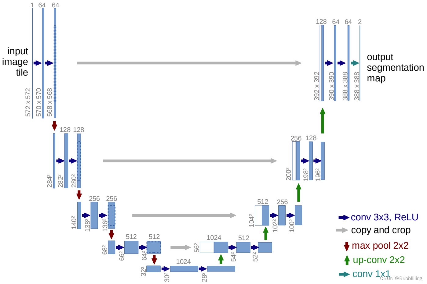
上图是典型的Unet模型结构,仅仅作为示意图,里面具体的数字同学们无需在意,和本文的学习无关。在本文中,Unet的输入和输出shape相同,通道均为3(一般为RGB三通道),宽高相同。
本质上,DDPM最重要的工作就是训练Unet模型,该模型输入为
x
t
x_t
xt和
t
t
t,输出为
x
t
−
1
x_{t-1}
xt−1时刻的**高斯噪声**。即利用
x
t
x_t
xt和
t
t
t预测上一时刻的高斯噪声。**这样就可以一步一步的再从噪声回到真实图像。**
假设我们需要生成一个[64, 64, 3]的图像,在
t
t
t时刻,我们有一个
x
t
x_t
xt噪声图,该噪声图的的shape也为[64, 64, 3],我们将它和
t
t
t一起输入到Unet中。Unet的输出为
x
t
−
1
x_{t-1}
xt−1时刻的[64, 64, 3]的噪声。
实现代码如下,代码中的特征提取模块为残差结构,方便优化:
import math

import torch
import torch.nn as nn
import torch.nn.functional as F

defget_norm(norm, num_channels, num_groups):if norm =="in":return nn.InstanceNorm2d(num_channels, affine=True)elif norm =="bn":return nn.BatchNorm2d(num_channels)elif norm =="gn":return nn.GroupNorm(num_groups, num_channels)elif norm isNone:return nn.Identity()else:raise ValueError("unknown normalization type")#------------------------------------------##   计算时间步长的位置嵌入。#   一半为sin,一半为cos。#------------------------------------------#classPositionalEmbedding(nn.Module):def__init__(self, dim, scale=1.0):super().__init__()assert dim %2==0
        self.dim = dim
        self.scale = scale

    defforward(self, x):
        device      = x.device
        half_dim    = self.dim //2
        emb = math.log(10000)/ half_dim
        emb = torch.exp(torch.arange(half_dim, device=device)*-emb)# x * self.scale和emb外积
        emb = torch.outer(x * self.scale, emb)
        emb = torch.cat((emb.sin(), emb.cos()), dim=-1)return emb

#------------------------------------------##   下采样层,一个步长为2x2的卷积#------------------------------------------#classDownsample(nn.Module):def__init__(self, in_channels):super().__init__()

        self.downsample = nn.Conv2d(in_channels, in_channels,3, stride=2, padding=1)defforward(self, x, time_emb, y):if x.shape[2]%2==1:raise ValueError("downsampling tensor height should be even")if x.shape[3]%2==1:raise ValueError("downsampling tensor width should be even")return self.downsample(x)#------------------------------------------##   上采样层,Upsample+卷积#------------------------------------------#classUpsample(nn.Module):def__init__(self, in_channels):super().__init__()
        self.upsample = nn.Sequential(
            nn.Upsample(scale_factor=2, mode="nearest"),
            nn.Conv2d(in_channels, in_channels,3, padding=1),)defforward(self, x, time_emb, y):return self.upsample(x)#------------------------------------------##   使用Self-Attention注意力机制#   做一个全局的Self-Attention#------------------------------------------#classAttentionBlock(nn.Module):def__init__(self, in_channels, norm="gn", num_groups=32):super().__init__()

        self.in_channels = in_channels
        self.norm = get_norm(norm, in_channels, num_groups)
        self.to_qkv = nn.Conv2d(in_channels, in_channels *3,1)
        self.to_out = nn.Conv2d(in_channels, in_channels,1)defforward(self, x):
        b, c, h, w  = x.shape
        q, k, v     = torch.split(self.to_qkv(self.norm(x)), self.in_channels, dim=1)

        q = q.permute(0,2,3,1).view(b, h * w, c)
        k = k.view(b, c, h * w)
        v = v.permute(0,2,3,1).view(b, h * w, c)

        dot_products = torch.bmm(q, k)*(c **(-0.5))assert dot_products.shape ==(b, h * w, h * w)

        attention   = torch.softmax(dot_products, dim=-1)
        out         = torch.bmm(attention, v)assert out.shape ==(b, h * w, c)
        out         = out.view(b, h, w, c).permute(0,3,1,2)return self.to_out(out)+ x

#------------------------------------------##   用于特征提取的残差结构#------------------------------------------#classResidualBlock(nn.Module):def__init__(
        self, in_channels, out_channels, dropout, time_emb_dim=None, num_classes=None, activation=F.relu,
        norm="gn", num_groups=32, use_attention=False,):super().__init__()

        self.activation = activation

        self.norm_1 = get_norm(norm, in_channels, num_groups)
        self.conv_1 = nn.Conv2d(in_channels, out_channels,3, padding=1)

        self.norm_2 = get_norm(norm, out_channels, num_groups)
        self.conv_2 = nn.Sequential(
            nn.Dropout(p=dropout),
            nn.Conv2d(out_channels, out_channels,3, padding=1),)

        self.time_bias  = nn.Linear(time_emb_dim, out_channels)if time_emb_dim isnotNoneelseNone
        self.class_bias = nn.Embedding(num_classes, out_channels)if num_classes isnotNoneelseNone

        self.residual_connection    = nn.Conv2d(in_channels, out_channels,1)if in_channels != out_channels else nn.Identity()
        self.attention              = nn.Identity()ifnot use_attention else AttentionBlock(out_channels, norm, num_groups)defforward(self, x, time_emb=None, y=None):
        out = self.activation(self.norm_1(x))# 第一个卷积
        out = self.conv_1(out)# 对时间time_emb做一个全连接,施加在通道上if self.time_bias isnotNone:if time_emb isNone:raise ValueError("time conditioning was specified but time_emb is not passed")
            out += self.time_bias(self.activation(time_emb))[:,:,None,None]# 对种类y_emb做一个全连接,施加在通道上if self.class_bias isnotNone:if y isNone:raise ValueError("class conditioning was specified but y is not passed")

            out += self.class_bias(y)[:,:,None,None]

        out = self.activation(self.norm_2(out))# 第二个卷积+残差边
        out = self.conv_2(out)+ self.residual_connection(x)# 最后做个Attention
        out = self.attention(out)return out

#------------------------------------------##   Unet模型#------------------------------------------#classUNet(nn.Module):def__init__(
        self, img_channels, base_channels=128, channel_mults=(1,2,2,2),
        num_res_blocks=2, time_emb_dim=128*4, time_emb_scale=1.0, num_classes=None, activation=F.silu,
        dropout=0.1, attention_resolutions=(1,), norm="gn", num_groups=32, initial_pad=0,):super().__init__()# 使用到的激活函数,一般为SILU
        self.activation = activation
        # 是否对输入进行padding
        self.initial_pad = initial_pad
        # 需要去区分的类别数
        self.num_classes = num_classes

        # 对时间轴输入的全连接层
        self.time_mlp = nn.Sequential(
            PositionalEmbedding(base_channels, time_emb_scale),
            nn.Linear(base_channels, time_emb_dim),
            nn.SiLU(),
            nn.Linear(time_emb_dim, time_emb_dim),)if time_emb_dim isnotNoneelseNone# 对输入图片的第一个卷积
        self.init_conv  = nn.Conv2d(img_channels, base_channels,3, padding=1)# self.downs用于存储下采样用到的层,首先利用ResidualBlock提取特征# 然后利用Downsample降低特征图的高宽
        self.downs      = nn.ModuleList()
        self.ups        = nn.ModuleList()# channels指的是每一个模块处理后的通道数# now_channels是一个中间变量,代表中间的通道数
        channels        =[base_channels]
        now_channels    = base_channels
        for i, mult inenumerate(channel_mults):
            out_channels = base_channels * mult
            for _ inrange(num_res_blocks):
                self.downs.append(
                    ResidualBlock(
                        now_channels, out_channels, dropout,
                        time_emb_dim=time_emb_dim, num_classes=num_classes, activation=activation,
                        norm=norm, num_groups=num_groups, use_attention=i in attention_resolutions,))
                now_channels = out_channels
                channels.append(now_channels)if i !=len(channel_mults)-1:
                self.downs.append(Downsample(now_channels))
                channels.append(now_channels)# 可以看作是特征整合,中间的一个特征提取模块
        self.mid = nn.ModuleList([
                ResidualBlock(
                    now_channels, now_channels, dropout,
                    time_emb_dim=time_emb_dim, num_classes=num_classes, activation=activation,
                    norm=norm, num_groups=num_groups, use_attention=True,),
                ResidualBlock(
                    now_channels, now_channels, dropout,
                    time_emb_dim=time_emb_dim, num_classes=num_classes, activation=activation,
                    norm=norm, num_groups=num_groups, use_attention=False,),])# 进行上采样,进行特征融合for i, mult inreversed(list(enumerate(channel_mults))):
            out_channels = base_channels * mult

            for _ inrange(num_res_blocks +1):
                self.ups.append(ResidualBlock(
                    channels.pop()+ now_channels, out_channels, dropout,
                    time_emb_dim=time_emb_dim, num_classes=num_classes, activation=activation,
                    norm=norm, num_groups=num_groups, use_attention=i in attention_resolutions,))
                now_channels = out_channels

            if i !=0:
                self.ups.append(Upsample(now_channels))assertlen(channels)==0

        self.out_norm = get_norm(norm, base_channels, num_groups)
        self.out_conv = nn.Conv2d(base_channels, img_channels,3, padding=1)defforward(self, x, time=None, y=None):# 是否对输入进行padding
        ip = self.initial_pad
        if ip !=0:
            x = F.pad(x,(ip,)*4)# 对时间轴输入的全连接层if self.time_mlp isnotNone:if time isNone:raise ValueError("time conditioning was specified but tim is not passed")
            time_emb = self.time_mlp(time)else:
            time_emb =Noneif self.num_classes isnotNoneand y isNone:raise ValueError("class conditioning was specified but y is not passed")# 对输入图片的第一个卷积
        x = self.init_conv(x)# skips用于存放下采样的中间层
        skips =[x]for layer in self.downs:
            x = layer(x, time_emb, y)
            skips.append(x)# 特征整合与提取for layer in self.mid:
            x = layer(x, time_emb, y)# 上采样并进行特征融合for layer in self.ups:ifisinstance(layer, ResidualBlock):
                x = torch.cat([x, skips.pop()], dim=1)
            x = layer(x, time_emb, y)# 上采样并进行特征融合
        x = self.activation(self.out_norm(x))
        x = self.out_conv(x)if self.initial_pad !=0:return x[:,:, ip:-ip, ip:-ip]else:return x
三、Diffusion的训练思路
Diffusion的训练思路比较简单,首先随机给每个batch里每张图片都生成一个t,代表我选择这个batch里面第t个时刻的噪声进行拟合。代码如下:
t = torch.randint(0, self.num_timesteps,(b,), device=device)
生成batch_size个噪声,计算施加这个噪声后模型在t个时刻的噪声图片是怎么样的,如下所示:
defperturb_x(self, x, t, noise):return(
        extract(self.sqrt_alphas_cumprod, t,  x.shape)* x +
        extract(self.sqrt_one_minus_alphas_cumprod, t, x.shape)* noise
    )defget_losses(self, x, t, y):# x, noise [batch_size, 3, 64, 64]
    noise           = torch.randn_like(x)

    perturbed_x     = self.perturb_x(x, t, noise)
之后利用这个噪声图片、t和网络模型计算预测噪声,利用预测噪声和实际噪声进行拟合。
defget_losses(self, x, t, y):# x, noise [batch_size, 3, 64, 64]
    noise           = torch.randn_like(x)

    perturbed_x     = self.perturb_x(x, t, noise)
    estimated_noise = self.model(perturbed_x, t, y)if self.loss_type =="l1":
        loss = F.l1_loss(estimated_noise, noise)elif self.loss_type =="l2":
        loss = F.mse_loss(estimated_noise, noise)return loss
利用DDPM生成图片
DDPM的库整体结构如下: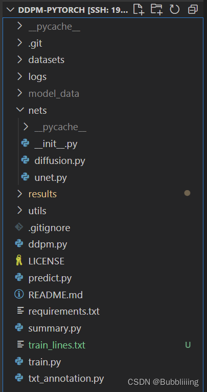
一、数据集的准备
在训练前需要准备好数据集,数据集保存在datasets文件夹里面。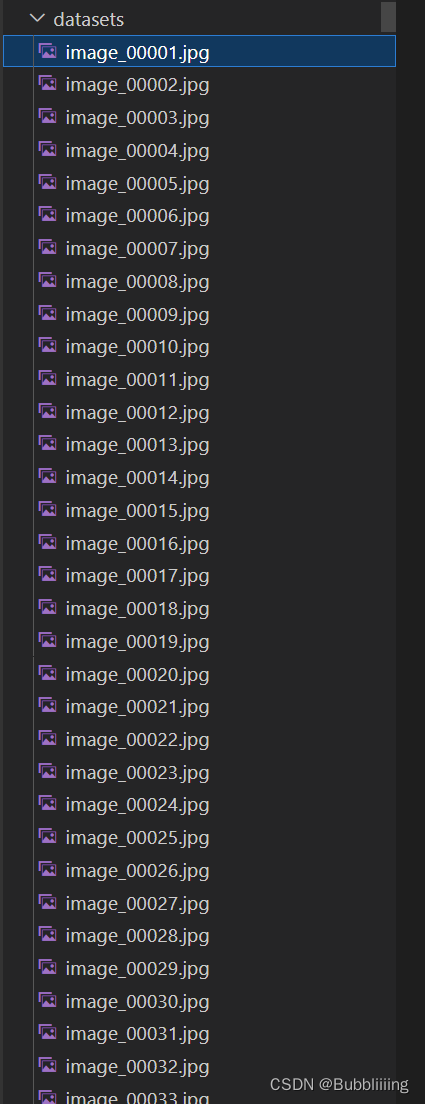
二、数据集的处理
打开txt_annotation.py,默认指向根目录下的datasets。运行txt_annotation.py。
此时生成根目录下面的train_lines.txt。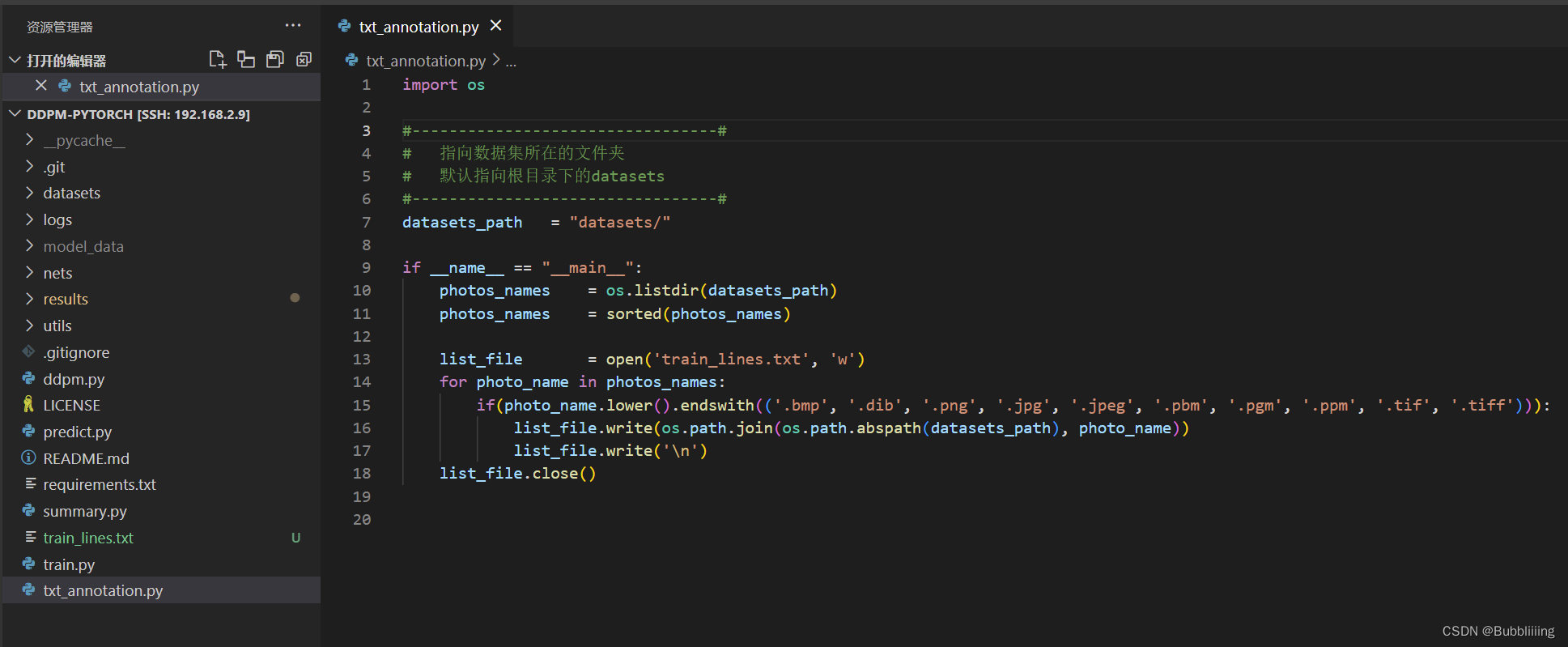
三、模型训练
在完成数据集处理后,运行train.py即可开始训练。
训练过程中,可在results文件夹内查看训练效果: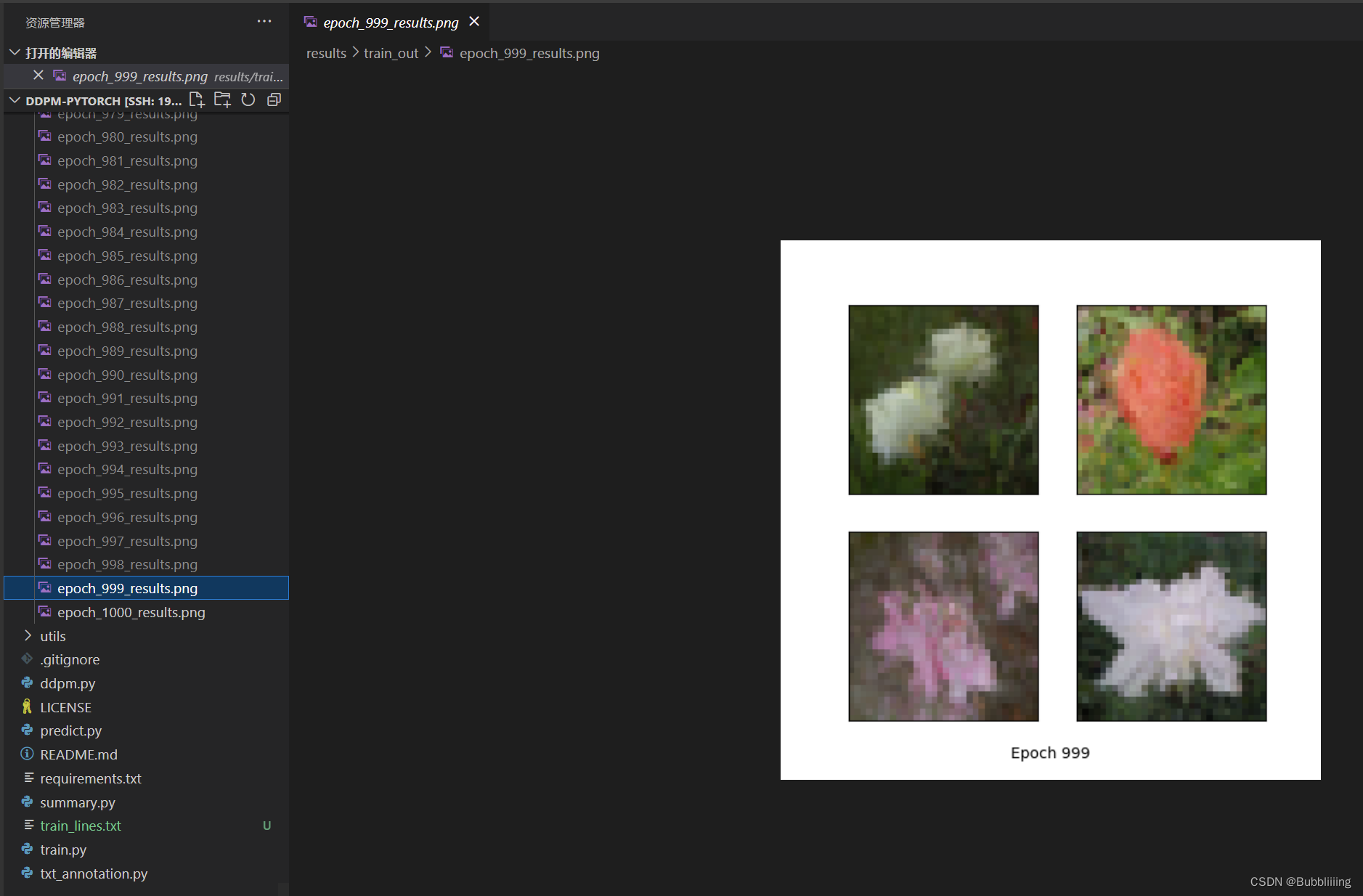
版权归原作者 Bubbliiiing 所有, 如有侵权,请联系我们删除。