GCN-图卷积神经网络算法简单实现（含python代码）

本文是就实现GCN算法模型进行的代码介绍，上一篇文章是GCN算法的原理和模型介绍。

代码中用到的Cora数据集：

链接：https://pan.baidu.com/s/1SbqIOtysKqHKZ7C50DM_eA
提取码：pfny

目的

本次实验的目的是将论文分类，通过模型训练，利用已经分好类的训练集，将论文通过GCN算法分为7类。

一、数据集介绍

数据集我选用的是GCN常用的Cora数据集，实验的目标就是通过对构造出来的两层GCN模型进行训练，实现对数据集样本节点的分类

Cora数据集下载地址：https://linqs-data.soe.ucsc.edu/public/lbc/cora.tgz

个人不建议用python的dgl包中的Cora数据，总是报错。

Cora数据集由关于机器学习方面的论文组成。 这些论文分为以下七个类别之一：

1.基于案例

2.遗传算法

3.神经网络

4.概率方法

5.强化学习

6.规则学习

7.理论

这些论文都是经过筛选的，在最终的数据集中，每篇论文引用或被至少一篇其他论文引用。整个语料库中有2708篇论文。

在词干堵塞和去除词尾后，只剩下1433个唯一的单词。文档频率小于10的所有单词都被删除。

即Cora数据集包含2708个顶点, 5429条边,每个顶点包含1433个特征，共有7个类别。

并且Cora已经把训练集和测试集的数据都划分好了，直接按照文件名读取数据即可，如

文件ind.cora.x => 训练实例的特征向量；ind.cora.y => 训练实例的标签，独热编码

ind.cora.tx => 测试实例的特征向量；ind.cora.ty => 测试实例的标签，独热编码

二、实现过程讲解

结合我最后做的代码实现，给大家先举一个引文网络的简单实例，方便大家了解处理过程。

其中每个节点代表一篇研究论文，同时边代表的是引用关系。

我们在这里有一个预处理步骤。在这里我们不使用原始论文作为特征，而是将论文转换成向量（通过使用NLP嵌入，例如tf-idf）。

假设我们使用average()函数（实际上GCN内部的传递函数肯定不是平均值，这里只是方便理解）。我们将对所有的节点进行同样的获取特征向量的操作。最后，我们将这些计算得到的平均值输入到神经网络中。

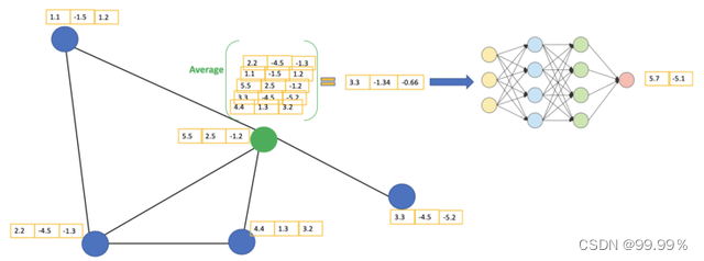
让我们考虑下绿色节点。首先，我们得到它的所有邻居的特征值，包括自身节点，接着取平均值。最后通过神经网络返回一个结果向量并将此作为最终结果。请注意，在GCN中，我们仅仅使用一个全连接层。在这个例子中，我们得到2维向量作为输出（全连接层的2个节点）。

全连接网络的作用就是对上一层得到的向量做乘法，最终降低其维度，然后输入到softmax层中得到对应的每个类别的得分。

在实际操作中，我们肯定是使用比average函数更复杂的聚合函数，也就是上面讲的那个传播函数。

我们还可以将更多的层叠加在一起，以获得更深的GCN。其中每一层的输出会被视为下一层的输入。

2层GCN的例子：第一层的输出是第二层的输入。

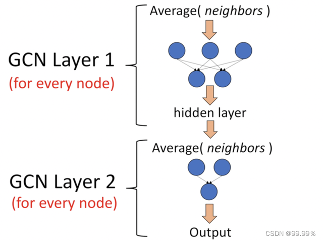
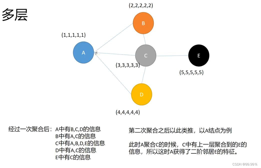
那么两层的GCN就可以在降维的同时，通过层间传播的公式获取到二阶邻居节点的特征：

在节点分类问题中，实际上在输入的邻接矩阵和每个节点的特征中，既包含了节点间的联系情况，也包含了节点自身的特征。

通过GCN的卷积层就可以实现降维，想要聚成几类就降成几维。

三、代码实现和结果分析

1. 导入包

import itertools
import os
import os.path as osp
import pickle
import urllib
from collections import namedtuple
import warnings
warnings.filterwarnings("ignore")
import numpy as np
import scipy.sparse as sp
import torch
import torch.nn as nn
import torch.nn.functional as F
import torch.nn.init as init
import torch.optim as optim
import matplotlib.pyplot as plt
%matplotlib inline

2. 数据准备¶

Data = namedtuple('Data', ['x', 'y', 'adjacency',
                           'train_mask', 'val_mask', 'test_mask'])

def tensor_from_numpy(x, device):
    return torch.from_numpy(x).to(device)

class CoraData(object):
    filenames = ["ind.cora.{}".format(name) for name in
                 ['x', 'tx', 'allx', 'y', 'ty', 'ally', 'graph', 'test.index']]

    def __init__(self, data_root="./data", rebuild=False):
        """Cora数据，包括数据下载，处理，加载等功能
        当数据的缓存文件存在时，将使用缓存文件，否则将下载、进行处理，并缓存到磁盘

        处理之后的数据可以通过属性 .data 获得，它将返回一个数据对象，包括如下几部分：
            * x: 节点的特征，维度为 2708 * 1433，类型为 np.ndarray
            * y: 节点的标签，总共包括7个类别，类型为 np.ndarray
            * adjacency: 邻接矩阵，维度为 2708 * 2708，类型为 scipy.sparse.coo.coo_matrix
            * train_mask: 训练集掩码向量，维度为 2708，当节点属于训练集时，相应位置为True，否则False
            * val_mask: 验证集掩码向量，维度为 2708，当节点属于验证集时，相应位置为True，否则False
            * test_mask: 测试集掩码向量，维度为 2708，当节点属于测试集时，相应位置为True，否则False

        Args:
        -------
            data_root: string, optional
                存放数据的目录，原始数据路径: ../data/cora
                缓存数据路径: {data_root}/ch5_cached.pkl
            rebuild: boolean, optional
                是否需要重新构建数据集，当设为True时，如果存在缓存数据也会重建数据

        """
        self.data_root = data_root #数据存放的路径
        save_file = osp.join(self.data_root, "ch5_cached.pkl")
        if osp.exists(save_file) and not rebuild:
            print("Using Cached file: {}".format(save_file))
            self._data = pickle.load(open(save_file, "rb"))
        else:
            self._data = self.process_data()
            with open(save_file, "wb") as f:
                pickle.dump(self.data, f)
            print("Cached file: {}".format(save_file))
    
    @property
    def data(self):
        """返回Data数据对象，包括x, y, adjacency, train_mask, val_mask, test_mask"""
        return self._data

    def process_data(self):
        """
        处理数据，得到节点特征和标签，邻接矩阵，训练集、验证集以及测试集
        引用自：https://github.com/rusty1s/pytorch_geometric
        """
        print("Process data ...")
        _, tx, allx, y, ty, ally, graph, test_index = [self.read_data(
            osp.join(self.data_root, name)) for name in self.filenames]
        train_index = np.arange(y.shape[0])
        val_index = np.arange(y.shape[0], y.shape[0] + 500)
        sorted_test_index = sorted(test_index)

        x = np.concatenate((allx, tx), axis=0)                #节点特征
        y = np.concatenate((ally, ty), axis=0).argmax(axis=1) #标签

        x[test_index] = x[sorted_test_index]
        y[test_index] = y[sorted_test_index]
        num_nodes = x.shape[0]

        train_mask = np.zeros(num_nodes, dtype=np.bool) #训练集
        val_mask = np.zeros(num_nodes, dtype=np.bool)   #验证集
        test_mask = np.zeros(num_nodes, dtype=np.bool)  #测试集
        train_mask[train_index] = True
        val_mask[val_index] = True
        test_mask[test_index] = True
        
        
        """"构建邻接矩阵"""
        adjacency = self.build_adjacency(graph)
        print("Node's feature shape: ", x.shape)
        print("Node's label shape: ", y.shape)
        print("Adjacency's shape: ", adjacency.shape)
        print("Number of training nodes: ", train_mask.sum())
        print("Number of validation nodes: ", val_mask.sum())
        print("Number of test nodes: ", test_mask.sum())

        return Data(x=x, y=y, adjacency=adjacency,
                    train_mask=train_mask, val_mask=val_mask, test_mask=test_mask)

    @staticmethod
    def build_adjacency(adj_dict):
        """根据邻接表创建邻接矩阵"""
        edge_index = []
        num_nodes = len(adj_dict)
        for src, dst in adj_dict.items():
            edge_index.extend([src, v] for v in dst)
            edge_index.extend([v, src] for v in dst)
        # 去除重复的边
        edge_index = list(k for k, _ in itertools.groupby(sorted(edge_index)))
        edge_index = np.asarray(edge_index)
        adjacency = sp.coo_matrix((np.ones(len(edge_index)), 
                                   (edge_index[:, 0], edge_index[:, 1])),
                    shape=(num_nodes, num_nodes), dtype="float32")
        return adjacency

    @staticmethod
    def read_data(path):
        """使用不同的方式读取原始数据以进一步处理"""
        name = osp.basename(path)
        if name == "ind.cora.test.index":
            out = np.genfromtxt(path, dtype="int64")
            return out
        else:
            out = pickle.load(open(path, "rb"), encoding="latin1")
            out = out.toarray() if hasattr(out, "toarray") else out
            return out

    @staticmethod
    def normalization(adjacency):
        """计算 H=D^-0.5 * (A+I) * D^-0.5"""
        adjacency += sp.eye(adjacency.shape[0])    # 增加自连接
        degree = np.array(adjacency.sum(1))
        d_hat = sp.diags(np.power(degree, -0.5).flatten())
        return d_hat.dot(adjacency).dot(d_hat).tocoo()

3. 图卷积层定义

class GraphConvolution(nn.Module):
    def __init__(self, input_dim, output_dim, use_bias=True):
        """图卷积：H*X*\theta

        Args:
        ----------
            input_dim: int
                节点输入特征的维度
            output_dim: int
                输出特征维度
            use_bias : bool, optional
                是否使用偏置
        """
        super(GraphConvolution, self).__init__()
        self.input_dim = input_dim
        self.output_dim = output_dim
        self.use_bias = use_bias
        self.weight = nn.Parameter(torch.Tensor(input_dim, output_dim))
        if self.use_bias:
            self.bias = nn.Parameter(torch.Tensor(output_dim))
        else:
            self.register_parameter('bias', None)
        self.reset_parameters() #初始化w

    def reset_parameters(self):
        init.kaiming_uniform_(self.weight) 
        #init.kaiming_uniform_神经网络权重初始化，神经网络要优化一个非常复杂的非线性模型，而且基本没有全局最优解，
        #初始化在其中扮演着非常重要的作用，尤其在没有BN等技术的早期，它直接影响模型能否收敛。
        
        if self.use_bias:
            init.zeros_(self.bias)

    def forward(self, adjacency, input_feature):
        """邻接矩阵是稀疏矩阵，因此在计算时使用稀疏矩阵乘法
    
        Args: 
        -------
            adjacency: torch.sparse.FloatTensor
                邻接矩阵
            input_feature: torch.Tensor
                输入特征
        """
        support = torch.mm(input_feature, self.weight)
        output = torch.sparse.mm(adjacency, support)
        if self.use_bias:
            output += self.bias
        return output

    def __repr__(self):
        return self.__class__.__name__ + ' (' \
            + str(self.input_dim) + ' -> ' \
            + str(self.output_dim) + ')'

4. GCN图卷积神经网络模型定义

有了数据和GCN层，就可以构建模型进行训练了。
定义一个两层的GCN，其中输入的维度为1433，隐藏层维度设为16，最后一层GCN将输出维度变为类别数7，激活函数使用的是ReLU。

class GcnNet(nn.Module):
    """
    定义一个包含两层GraphConvolution的模型
    """
    def __init__(self, input_dim=1433):
        super(GcnNet, self).__init__()
        self.gcn1 = GraphConvolution(input_dim, 16)
        self.gcn2 = GraphConvolution(16, 7)
    
    def forward(self, adjacency, feature):
        h = F.relu(self.gcn1(adjacency, feature))
        logits = self.gcn2(adjacency, h)
        return logits

5. 模型训练

5.1 超参数定义，包含学习率、正则化系数等。

LEARNING_RATE = 0.1 #学习率 学习率过小→ →→收敛过慢，学习率过大→ →→错过局部最优；
WEIGHT_DACAY = 5e-4 #正则化系数 weight_dacay，解决过拟合问题
EPOCHS = 200        #完整遍历训练集的次数
DEVICE = "cuda" if torch.cuda.is_available() else "cpu" #指定设备，如果当前显卡忙于其他工作，可以设置为 DEVICE = "cpu"，使用cpu运行

为什么要训练200轮呢，因为我们最开始是不知道边的权重的，需要通过模型训练出来合适的权重，也就是公式中的W。

# 加载数据，并转换为torch.Tensor
dataset = CoraData().data
node_feature = dataset.x / dataset.x.sum(1, keepdims=True)  # 归一化数据，使得每一行和为1
tensor_x = tensor_from_numpy(node_feature, DEVICE)
tensor_y = tensor_from_numpy(dataset.y, DEVICE)
tensor_train_mask = tensor_from_numpy(dataset.train_mask, DEVICE)
tensor_val_mask = tensor_from_numpy(dataset.val_mask, DEVICE)
tensor_test_mask = tensor_from_numpy(dataset.test_mask, DEVICE)
normalize_adjacency = CoraData.normalization(dataset.adjacency)   # 规范化邻接矩阵

num_nodes, input_dim = node_feature.shape
indices = torch.from_numpy(np.asarray([normalize_adjacency.row, 
                                       normalize_adjacency.col]).astype('int64')).long()
values = torch.from_numpy(normalize_adjacency.data.astype(np.float32))
tensor_adjacency = torch.sparse.FloatTensor(indices, values, 
                                            (num_nodes, num_nodes)).to(DEVICE)

5.2 定义模型：

# 模型定义：Model, Loss, Optimizer
model = GcnNet(input_dim).to(DEVICE)
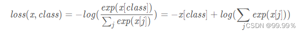
criterion = nn.CrossEntropyLoss().to(DEVICE) #nn.CrossEntropyLoss()函数计算交叉熵损失
optimizer = optim.Adam(model.parameters(), 
                       lr=LEARNING_RATE, 
                       weight_decay=WEIGHT_DACAY)

其中在定义模型时，还顺手定义了criterion，即在训练过程中可以用nn.CrossEntropyLoss()函数计算交叉熵损失：

5.3 定义训练和测试函数，进行训练

# 训练主体函数
def train():
    loss_history = []
    val_acc_history = []
    model.train()
    train_y = tensor_y[tensor_train_mask]
    
    for epoch in range(EPOCHS):
        # 共进行200次训练
        logits = model(tensor_adjacency, tensor_x)  # 前向传播
        #其中logits是模型输出，tensor_adjacency, tensor_x分别是邻接矩阵和节点特征。
        
        train_mask_logits = logits[tensor_train_mask]   # 只选择训练节点进行监督
        loss = criterion(train_mask_logits, train_y)    # 计算损失值，目的是优化模型，获得更科学的权重W
        optimizer.zero_grad()
        loss.backward()     # 反向传播计算参数的梯度
        optimizer.step()    # 使用优化方法进行梯度更新
        train_acc, _, _ = test(tensor_train_mask)     # 计算当前模型训练集上的准确率
        val_acc, _, _ = test(tensor_val_mask)     # 计算当前模型在验证集上的准确率
        
        # 记录训练过程中损失值和准确率的变化，用于画图
        loss_history.append(loss.item())
        val_acc_history.append(val_acc.item())
        print("Epoch {:03d}: Loss {:.4f}, TrainAcc {:.4}, ValAcc {:.4f}".format(
            epoch, loss.item(), train_acc.item(), val_acc.item()))
    
    return loss_history, val_acc_history

# 测试函数
def test(mask):
    model.eval()  # 表示将模型转变为evaluation（测试）模式，这样就可以排除BN和Dropout对测试的干扰
    
    with torch.no_grad():  # 显著减少显存占用
        logits = model(tensor_adjacency, tensor_x) #(N,16)->(N,7) N节点数
        test_mask_logits = logits[mask]  # 矩阵形状和mask一样
        
        predict_y = test_mask_logits.max(1)[1]  # 返回每一行的最大值中索引（返回最大元素在各行的列索引）
        accuarcy = torch.eq(predict_y, tensor_y[mask]).float().mean()
    return accuarcy, test_mask_logits.cpu().numpy(), tensor_y[mask].cpu().numpy()

使用上述代码进行模型训练，可以看到如下代码所示的日志输出:

loss, val_acc = train()
test_acc, test_logits, test_label = test(tensor_test_mask)
print("Test accuarcy: ", test_acc.item())#item()返回的是一个浮点型数据，测试集准确率

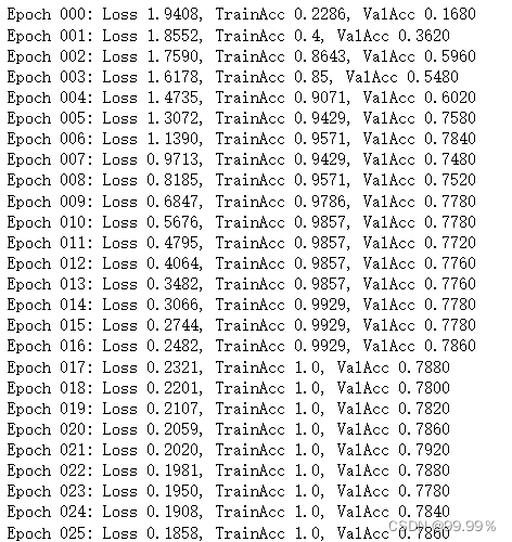
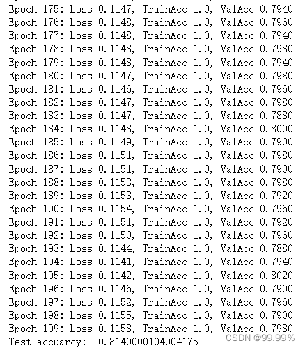
其中Epoch为训练轮数；loss是损失值；TrainAcc训练集准确率；ValAcc测试集上的准确率；

6. 可视化

将损失值和验证集准确率的变化趋势可视化：

损失函数用来测度模型的输出值和真实因变量值之间的差异

def plot_loss_with_acc(loss_history, val_acc_history):
    fig = plt.figure()
    # 坐标系ax1画曲线1
    ax1 = fig.add_subplot(111)  # 指的是将plot界面分成1行1列，此子图占据从左到右从上到下的1位置
    ax1.plot(range(len(loss_history)), loss_history,
             c=np.array([255, 71, 90]) / 255.)  # c为颜色
    plt.ylabel('Loss')
    
    # 坐标系ax2画曲线2
    ax2 = fig.add_subplot(111, sharex=ax1, frameon=False)  # 其本质就是添加坐标系，设置共享ax1的x轴，ax2背景透明
    ax2.plot(range(len(val_acc_history)), val_acc_history,
             c=np.array([79, 179, 255]) / 255.)
    ax2.yaxis.tick_right()  # 开启右边的y坐标
    
    ax2.yaxis.set_label_position("right")
    plt.ylabel('ValAcc')
    
    plt.xlabel('Epoch')
    plt.title('Training Loss & Validation Accuracy')
    plt.show()

plot_loss_with_acc(loss, val_acc)

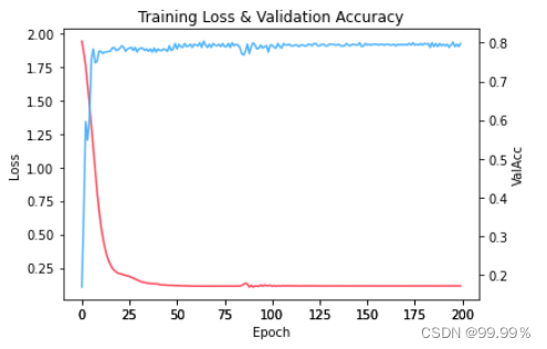
可以看到红线代表的损失值随着训练次数的增加越来越小，蓝线代表的模型准确率越来越高。

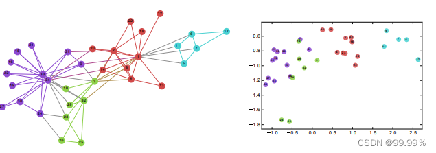
将最后一层得到的输出进行TSNE降维，（TSNE）t分布随机邻域嵌入 是一种用于探索高维数据的非线性降维算法。

它将多维数据映射到适合于人类观察的两个或多个维度。

得到如下图所示的分类结果：

绘制测试数据的TSNE降维图：

from sklearn.manifold import TSNE
tsne = TSNE()
out = tsne.fit_transform(test_logits)
fig = plt.figure()
for i in range(7):
    indices = test_label == i
    x, y = out[indices].T
    plt.scatter(x, y, label=str(i))
plt.legend()

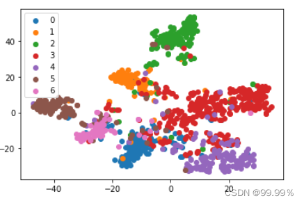
根据上述结果：我们通过图卷积神经网络算法，可以成功将论文集划分为较为鲜明的7类，这与论文集原本的种类划分基本一致，效果还是较为可观的。