Residual, BottleNeck, Inverted Residual, MBConv的解释和Pytorch实现

上篇ConvNext的文章有小伙伴问BottleNeck，Inverted Residual的区别，所以找了这篇文章，详细的解释一些用到的卷积块，当作趁热打铁吧

在介绍上面的这些概念之间，我们先创建一个通用的 conv-norm-act 层，这也是最基本的卷积块。

fromfunctoolsimportpartial
fromtorchimportnn
classConvNormAct(nn.Sequential):
    def__init__(
        self,
        in_features: int,
        out_features: int,
        kernel_size: int,
        norm: nn.Module = nn.BatchNorm2d,
        act: nn.Module = nn.ReLU,
        **kwargs
    ):
        super().__init__(
            nn.Conv2d(
                in_features,
                out_features,
                kernel_size=kernel_size,
                padding=kernel_size//2,
            ),
            norm(out_features),
            act(),
        )
Conv1X1BnReLU = partial(ConvNormAct, kernel_size=1)
Conv3X3BnReLU = partial(ConvNormAct, kernel_size=3)
importtorch
x = torch.randn((1, 32, 56, 56))
Conv1X1BnReLU(32, 64)(x).shape
#torch.Size([1, 64, 56, 56])

残差连接

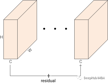
ResNet 中提出并使用了残差连接，这个想法是将层的输入与层的输出相加，输出 = 层（输入）+ 输入。下图可以帮助您将其可视化。但是，它只使用了一个 + 运算符。残差操作提高了梯度在乘法器层上传播的能力，允许有效地训练超过一百层的网络。

在PyTorch中，我们可以轻松地创建一个ResidualAdd层

fromtorchimportnn
fromtorchimportTensor
classResidualAdd(nn.Module):
    def__init__(self, block: nn.Module):
        super().__init__()
        self.block = block
        
    defforward(self, x: Tensor) ->Tensor:
        res = x
        x = self.block(x)
        x += res
        returnx
    
ResidualAdd(
    nn.Conv2d(32, 32, kernel_size=1)
)(x).shape

捷径 Shortcut

有时候残差没有相同的输出维度，所以无法将它们相加。所以就需要使用conv(带+的黑色箭头)来投影输入，以匹配输出的特性

fromtypingimportOptional
classResidualAdd(nn.Module):
    def__init__(self, block: nn.Module, shortcut: Optional[nn.Module] = None):
        super().__init__()
        self.block = block
        self.shortcut = shortcut
        
    defforward(self, x: Tensor) ->Tensor:
        res = x
        x = self.block(x)
        ifself.shortcut:
            res = self.shortcut(res)
        x += res
        returnx
ResidualAdd(
    nn.Conv2d(32, 64, kernel_size=1),
    shortcut=nn.Conv2d(32, 64, kernel_size=1)
)(x).shape

瓶颈块 BottleNeck

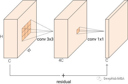
在用于图像识别的深度残差网络中也引入了瓶颈块。BottleNeck 块接受大小为 BxCxHxW 的输入，它首先使用1x1 卷积将其缩减为 BxC/rxHxW，然后再应用 3x3 卷积，最后再使用 1x1 卷积将输出重新映射到与输入相同的特征维度BxCxHxW 。这比使用三个 3x3 转换要快的多，由于中间层减少输入维度，所以将其称之为“BottleNeck”。下图可视化了该块，我们在原始实现中使用 r=4

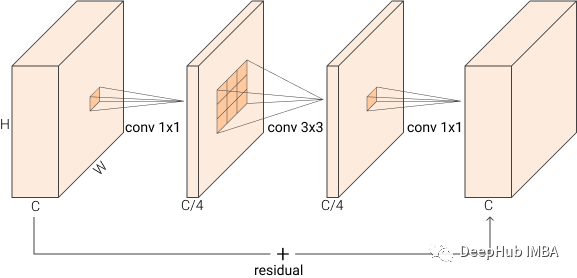
前两个convs之后是batchnorm和一个非线性激活，在加法之后还有一个非线性的激活

fromtorchimportnn
classBottleNeck(nn.Sequential):
    def__init__(self, in_features: int, out_features: int, reduction: int = 4):
        reduced_features = out_features//reduction
        super().__init__(
            nn.Sequential(
                ResidualAdd(
                    nn.Sequential(
                        # wide -> narrow
                        Conv1X1BnReLU(in_features, reduced_features),
                        # narrow -> narrow
                        Conv3X3BnReLU(reduced_features, reduced_features),
                        # narrow -> wide
                        Conv1X1BnReLU(reduced_features, out_features, act=nn.Identity),
                    ),
                    shortcut=Conv1X1BnReLU(in_features, out_features)
                    ifin_features!= out_features
                    elseNone,
                ),
                nn.ReLU(),
            )
        )
        
BottleNeck(32, 64)(x).shape

请注意这里仅在输入和输出特征维度不同时才使用shortcut。

一般情况下当希望减少空间维度时，在中间卷积中使用 stride=2。

线性瓶颈 Linear BottleNeck

线性瓶颈是在 MobileNetV2: Inverted Residuals 中引入的。线性瓶颈块是不包含最后一个激活的瓶颈块。在论文的第 3.2 节中，他们详细介绍了为什么在输出之前存在非线性会损害性能。简而言之：非线性函数 Line ReLU 将所有 < 0 设置为 0会破坏信息。根据经验表明，当输入的通道小于输出的通道时删除最后的激活函数是正确的。所以只要删除 BottleNeck 中的 nn.ReLU 即可。

倒置残差 Inverted Residual

在 MobileNetV2 中还引入了倒置残差。Inverted Residual 块是倒置的 BottleNeck 层。他们使用第一个 conv 对维度进行扩展而不是减少。下图应该清楚地说明这一点

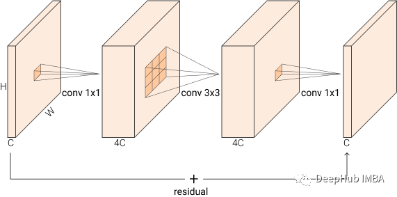
从 BxCxHxW -> BxCexHxW -> BxCexHxW -> BxCxHxW，其中 e 是膨胀比，默认设置为 4。而不是像正常的瓶颈块那样变宽 -> 窄 -> 宽，他们做相反的事情窄 -> 宽 -> 窄。

classInvertedResidual(nn.Sequential):
    def__init__(self, in_features: int, out_features: int, expansion: int = 4):
        expanded_features = in_features*expansion
        super().__init__(
            nn.Sequential(
                ResidualAdd(
                    nn.Sequential(
                        # narrow -> wide
                        Conv1X1BnReLU(in_features, expanded_features),
                        # wide -> wide
                        Conv3X3BnReLU(expanded_features, expanded_features),
                        # wide -> narrow
                        Conv1X1BnReLU(expanded_features, out_features, act=nn.Identity),
                    ),
                    shortcut=Conv1X1BnReLU(in_features, out_features)
                    ifin_features!= out_features
                    elseNone,
                ),
                nn.ReLU(),
            )
        )
        
InvertedResidual(32, 64)(x).shape

在 MobileNet 中，残差连接仅在输入和输出特征匹配时应用，这个我们在前面已经说明了

classMobileNetLikeBlock(nn.Sequential):
    def__init__(self, in_features: int, out_features: int, expansion: int = 4):
        # use ResidualAdd if features match, otherwise a normal Sequential
        residual = ResidualAddifin_features == out_featureselsenn.Sequential
        expanded_features = in_features*expansion
        super().__init__(
            nn.Sequential(
                residual(
                    nn.Sequential(
                        # narrow -> wide
                        Conv1X1BnReLU(in_features, expanded_features),
                        # wide -> wide
                        Conv3X3BnReLU(expanded_features, expanded_features),
                        # wide -> narrow
                        Conv1X1BnReLU(expanded_features, out_features, act=nn.Identity),
                    ),
                ),
                nn.ReLU(),
            )
        )
        
MobileNetLikeBlock(32, 64)(x).shape
MobileNetLikeBlock(32, 32)(x).shape

MBConv

在 MobileNetV2 之后，它的构建块被称为 MBConv。MBConv 是具有深度可分离卷积的倒置线性瓶颈层，听着很绕对吧，其实就是把上面我们介绍的几个块进行了整合。

1、深度可分离卷积 Depth-Wise Separable Convolutions

Depth-Wise Separable Convolutions 是一种减少参数的数量技巧，它将一个普通的 3x3 卷积拆分为两个卷积。第一个卷积将单个的 3x3 卷积核应用于每个输入的通道，另一个卷积将 1x1 卷积核应用于所有通道。这和做一个普通的 3x3 转换是一样的，但是却减少了参数。

但是其实这个有点多余，因为在我们现有的硬件上它比普通的 3x3 慢得多。

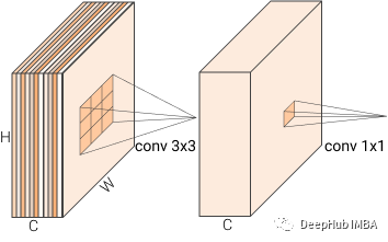
通道中的不同颜色代表每个通道应用的一个单独的卷积核（过滤器）

classDepthWiseSeparableConv(nn.Sequential):
    def__init__(self, in_features: int, out_features: int):
        super().__init__(
            nn.Conv2d(in_features, in_features, kernel_size=3, groups=in_features),
            nn.Conv2d(in_features, out_features, kernel_size=1)
        )
        
DepthWiseSeparableConv(32, 64)(x).shape

让我们看看参数减少了多少：

sum(p.numel() forpinDepthWiseSeparableConv(32, 64).parameters() ifp.requires_grad) 
#2432

再看看一个普通的 Conv2d

sum(p.numel() forpinnn.Conv2d(32, 64, kernel_size=3).parameters() ifp.requires_grad)
#18496

这是巨大的差距

2、完成MBConv

现在可以创建一个完整的 MBConv。MBConv 有几个重要细节，归一化适用于深度和点卷积，非线性仅适用于深度卷积（请记住线性瓶颈）。而激活函数使用ReLU6 。我们现在把把所有东西放在一起

classMBConv(nn.Sequential):
    def__init__(self, in_features: int, out_features: int, expansion: int = 4):
        residual = ResidualAddifin_features == out_featureselsenn.Sequential
        expanded_features = in_features*expansion
        super().__init__(
            nn.Sequential(
                residual(
                    nn.Sequential(
                        # narrow -> wide
                        Conv1X1BnReLU(in_features, 
                                      expanded_features,
                                      act=nn.ReLU6
                                     ),
                        # wide -> wide
                        Conv3X3BnReLU(expanded_features, 
                                      expanded_features, 
                                      groups=expanded_features,
                                      act=nn.ReLU6
                                     ),
                        # here you can apply SE
                        # wide -> narrow
                        Conv1X1BnReLU(expanded_features, out_features, act=nn.Identity),
                    ),
                ),
                nn.ReLU(),
            )
        )
        
MBConv(32, 64)(x).shape

在 EfficientNet 中也使用的是带有 Squeeze 和 Excitation的这个块的修改的版本。

融合倒置残差 (Fused MBConv)

在 EfficientNetV2: Smaller Models and Faster Training 中引入了 Fused Inverted Residuals，这样可以使 MBConv 更快。解决了我们上面说的深度卷积很慢的问题，它们将第一个和第二个卷积融合在一个 3x3 卷积中（第 3.2 节）。

classFusedMBConv(nn.Sequential):
    def__init__(self, in_features: int, out_features: int, expansion: int = 4):
        residual = ResidualAddifin_features == out_featureselsenn.Sequential
        expanded_features = in_features*expansion
        super().__init__(
            nn.Sequential(
                residual(
                    nn.Sequential(
                        Conv3X3BnReLU(in_features, 
                                      expanded_features, 
                                      act=nn.ReLU6
                                     ),
                        # here you can apply SE
                        # wide -> narrow
                        Conv1X1BnReLU(expanded_features, out_features, act=nn.Identity),
                    ),
                ),
                nn.ReLU(),
            )
        )
        
MBConv(32, 64)(x).shape

总结

本文介绍了这些基本的卷积块的操作和代码，这些卷积块的架构是我们在CV中经常会遇到的，所以强烈建议阅读与他们相关的论文。另外如果你对本文代码感兴趣，请看这里：

https://github.com/FrancescoSaverioZuppichini/BottleNeck-InvertedResidual-FusedMBConv-in-PyTorch/blob/main/README.ipynb

作者：Francesco Zuppichini

标签：深度学习计算机视觉神经网络

Residual, BottleNeck, Inverted Residual, MBConv的解释和Pytorch实现

残差连接

捷径 Shortcut

瓶颈块 BottleNeck

线性瓶颈 Linear BottleNeck

倒置残差 Inverted Residual

MBConv

融合倒置残差 (Fused MBConv)

总结

发表评论

“Residual, BottleNeck, Inverted Residual, MBConv的解释和Pytorch实现”的评论:

关于作者

Deephub

相关阅读

文章导航