
人体活动识别(HAR)是一种使用人工智能(AI)从智能手表等活动记录设备产生的原始数据中识别人类活动的方法。当人们执行某种动作时,人们佩戴的传感器(智能手表、手环、专用设备等)就会产生信号。这些收集信息的传感器包括加速度计、陀螺仪和磁力计。人类活动识别有各种各样的应用,从为病人和残疾人提供帮助到像游戏这样严重依赖于分析运动技能的领域。我们可以将这些人类活动识别技术大致分为两类:固定传感器和移动传感器。在本文中,我们使用移动传感器产生的原始数据来识别人类活动。

在本文中,我将使用LSTM (Long - term Memory)和CNN (Convolutional Neural Network)来识别下面的人类活动:
- 下楼
- 上楼
- 跑步
- 坐着
- 站立
- 步行
概述
你可能会考虑为什么我们要使用LSTM-CNN模型而不是基本的机器学习方法?
机器学习方法在很大程度上依赖于启发式手动特征提取人类活动识别任务,而我们这里需要做的是端到端的学习,简化了启发式手动提取特征的操作。
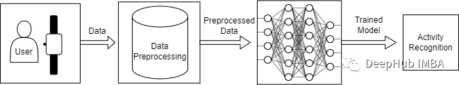
我将要使用的模型是一个深神经网络,该网络是LSTM和CNN的组合形成的,并且具有提取活动特征和仅使用模型参数进行分类的能力。
这里我们使用WISDM数据集,总计1.098.209样本。通过我们的训练,模型的F1得分为0.96,在测试集上,F1得分为0.89。
导入库
首先,我们将导入我们将需要的所有必要库。
from pandas import read_csv, unique

import numpy as np

from scipy.interpolate import interp1d
from scipy.stats import mode

from sklearn.preprocessing import LabelEncoder
from sklearn.metrics import classification_report, confusion_matrix, ConfusionMatrixDisplay

from tensorflow import stack
from tensorflow.keras.utils import to_categorical
from keras.models import Sequential
from keras.layers import Dense, GlobalAveragePooling1D, BatchNormalization, MaxPool1D, Reshape, Activation
from keras.layers import Conv1D, LSTM
from keras.callbacks import ModelCheckpoint, EarlyStopping
import matplotlib.pyplot as plt
%matplotlib inline

import warnings
warnings.filterwarnings("ignore")
我们将使用Sklearn,Tensorflow,Keras,Scipy和Numpy来构建模型和进行数据预处理。使用PANDAS 进行数据加载,使用matplotlib进行数据可视化。
数据集加载和可视化
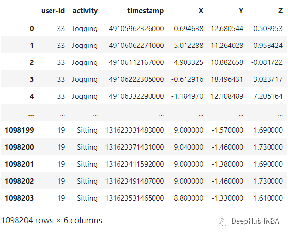
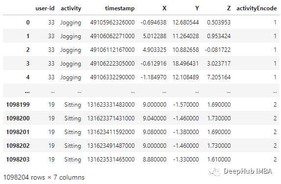
WISDM是由个人腰间携带的移动设备上的加速计记录下来。该数据收集是由个人监督的可以确保数据的质量。我们将使用的文件是WISDM_AR_V1.1_RAW.TXT。使用PANDAS,可以将数据集加载到DataAframe中,如下面代码:
def read_data(filepath):
    df = read_csv(filepath, header=None, names=['user-id',
                                               'activity',
                                               'timestamp',
                                               'X',
                                               'Y',
                                               'Z'])
    ## removing ';' from last column and converting it to float
    df['Z'].replace(regex=True, inplace=True, to_replace=r';', value=r'')
    df['Z'] = df['Z'].apply(convert_to_float)
    return df

def convert_to_float(x):
    try:
        return np.float64(x)
    except:
        return np.nan

df = read_data('Dataset/WISDM_ar_v1.1/WISDM_ar_v1.1_raw.txt')
df
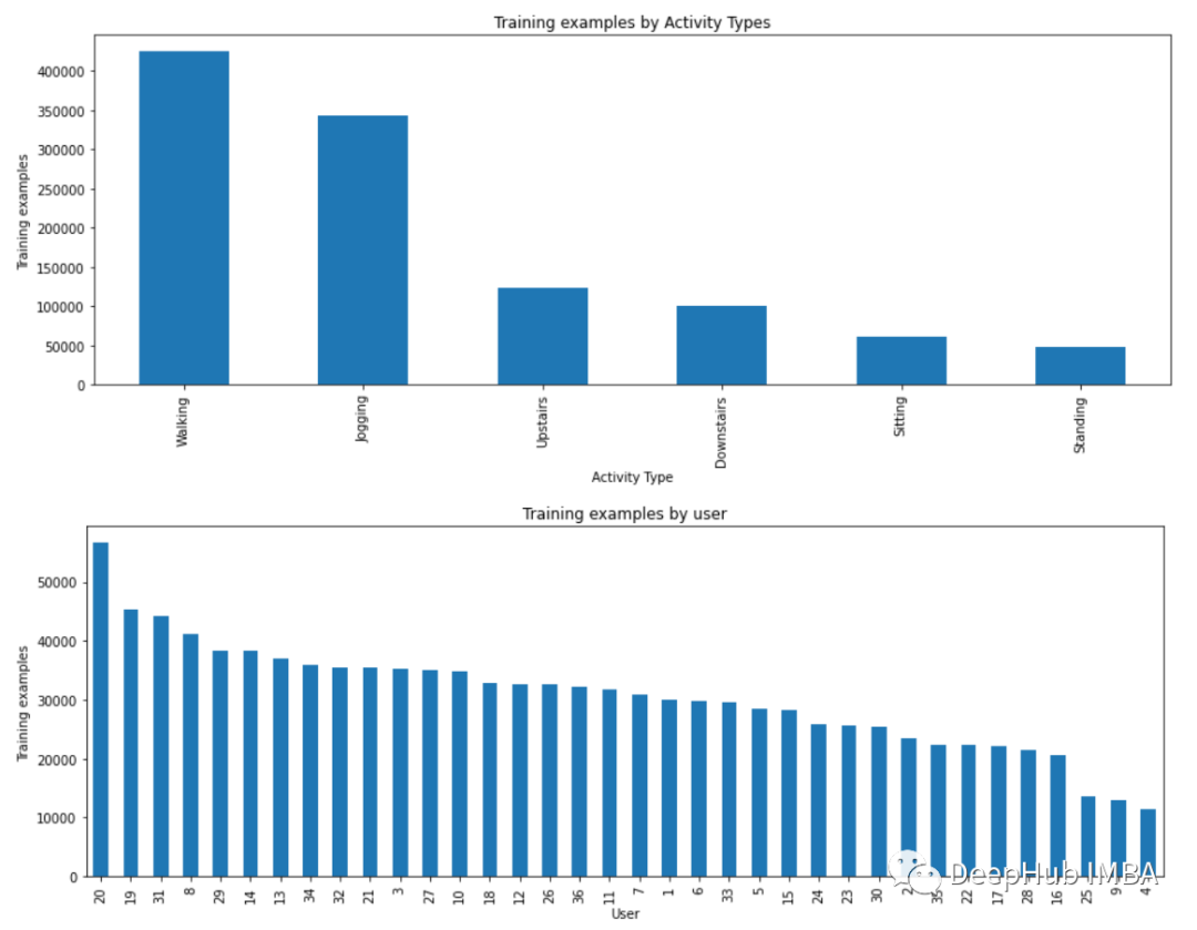
plt.figure(figsize=(15, 5))

plt.xlabel('Activity Type')
plt.ylabel('Training examples')
df['activity'].value_counts().plot(kind='bar',
                                  title='Training examples by Activity Types')
plt.show()

plt.figure(figsize=(15, 5))
plt.xlabel('User')
plt.ylabel('Training examples')
df['user-id'].value_counts().plot(kind='bar',
                                 title='Training examples by user')
plt.show()
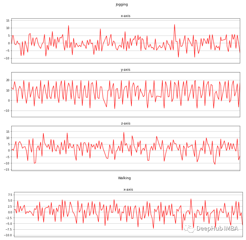
现在我将收集的三个轴上的加速度计数据进行可视化。
def axis_plot(ax, x, y, title):
    ax.plot(x, y, 'r')
    ax.set_title(title)
    ax.xaxis.set_visible(False)
    ax.set_ylim([min(y) - np.std(y), max(y) + np.std(y)])
    ax.set_xlim([min(x), max(x)])
    ax.grid(True)

for activity in df['activity'].unique():
    limit = df[df['activity'] == activity][:180]
    fig, (ax0, ax1, ax2) = plt.subplots(nrows=3, sharex=True, figsize=(15, 10))
    axis_plot(ax0, limit['timestamp'], limit['X'], 'x-axis')
    axis_plot(ax1, limit['timestamp'], limit['Y'], 'y-axis')
    axis_plot(ax2, limit['timestamp'], limit['Z'], 'z-axis')
    plt.subplots_adjust(hspace=0.2)
    fig.suptitle(activity)
    plt.subplots_adjust(top=0.9)
    plt.show()
数据预处理
数据预处理是一项非常重要的任务,它使我们的模型能够更好的利用我们的原始数据。这里将使用的数据预处理方法有:
- 标签编码
- 线性插值
- 数据分割
- 归一化
- 时间序列分割
- 独热编码
标签编码
由于模型不能接受非数字标签作为输入,我们将在另一列中添加' activity '列的编码标签,并将其命名为' activityEncode '。标签被转换成如下所示的数字标签(这个标签是我们要预测的结果标签)
- Downstairs [0]
- Jogging [1]
- Sitting [2]
- Standing [3]
- Upstairs [4]
- Walking [5]
label_encode = LabelEncoder()
df['activityEncode'] = label_encode.fit_transform(df['activity'].values.ravel())
df
线性插值
利用线性插值可以避免采集过程中出现NaN的数据丢失的问题。它将通过插值法填充缺失的值。虽然在这个数据集中只有一个NaN值,但为了我们的展示,还是需要实现它。
interpolation_fn = interp1d(df['activityEncode'] ,df['Z'], kind='linear')
null_list = df[df['Z'].isnull()].index.tolist()
for i in null_list:
    y = df['activityEncode'][i]
    value = interpolation_fn(y)
    df['Z']=df['Z'].fillna(value)
    print(value)
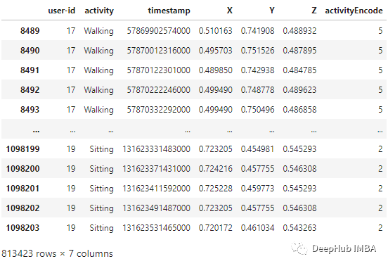
数据分割
根据用户id进行数据分割,避免数据分割错误。我们在训练集中使用id小于或等于27的用户,其余的在测试集中使用。
df_test = df[df['user-id'] > 27]
df_train = df[df['user-id'] <= 27]
归一化
在训练之前,需要将数据特征归一化到0到1的范围内。我们用的方法是
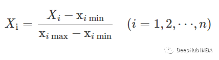
df_train['X'] = (df_train['X']-df_train['X'].min())/(df_train['X'].max()-df_train['X'].min())
df_train['Y'] = (df_train['Y']-df_train['Y'].min())/(df_train['Y'].max()-df_train['Y'].min())
df_train['Z'] = (df_train['Z']-df_train['Z'].min())/(df_train['Z'].max()-df_train['Z'].min())
df_train
时间序列分割
因为我们处理的是时间序列数据, 所以需要创建一个分割的函数,标签名称和每个记录的范围进行分段。此函数在x_train和y_train中执行特征的分离,将每80个时间段分成一组数据。
def segments(df, time_steps, step, label_name):
    N_FEATURES = 3
    segments = []
    labels = []
    for i in range(0, len(df) - time_steps, step):
        xs = df['X'].values[i:i+time_steps]
        ys = df['Y'].values[i:i+time_steps]
        zs = df['Z'].values[i:i+time_steps]

        label = mode(df[label_name][i:i+time_steps])[0][0]
        segments.append([xs, ys, zs])
        labels.append(label)

    reshaped_segments = np.asarray(segments, dtype=np.float32).reshape(-1, time_steps, N_FEATURES)
    labels = np.asarray(labels)

    return reshaped_segments, labels

TIME_PERIOD = 80
STEP_DISTANCE = 40
LABEL = 'activityEncode'
x_train, y_train = segments(df_train, TIME_PERIOD, STEP_DISTANCE, LABEL)
这样,x_train和y_train形状变为:
print('x_train shape:', x_train.shape)
print('Training samples:', x_train.shape[0])
print('y_train shape:', y_train.shape)

x_train shape: (20334, 80, 3)
Training samples: 20334
y_train shape: (20334,)
这里还存储了一些后面用到的数据:时间段(time_period),传感器数(sensors)和类(num_classes)的数量。
time_period, sensors = x_train.shape[1], x_train.shape[2]
num_classes = label_encode.classes_.size
print(list(label_encode.classes_))

['Downstairs', 'Jogging', 'Sitting', 'Standing', 'Upstairs', 'Walking']
最后需要使用Reshape将其转换为列表,作为keras的输入
input_shape = time_period * sensors
x_train = x_train.reshape(x_train.shape[0], input_shape)
print("Input Shape: ", input_shape)
print("Input Data Shape: ", x_train.shape)

Input Shape:  240
Input Data Shape:  (20334, 240)
最后需要将所有数据转换为float32。
x_train = x_train.astype('float32')
y_train = y_train.astype('float32')
独热编码
这是数据预处理的最后一步,我们将通过编码标签并将其存储到y_train_hot中来执行。
y_train_hot = to_categorical(y_train, num_classes)
print("y_train shape: ", y_train_hot.shape)
y_train shape:  (20334, 6)
模型
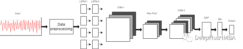
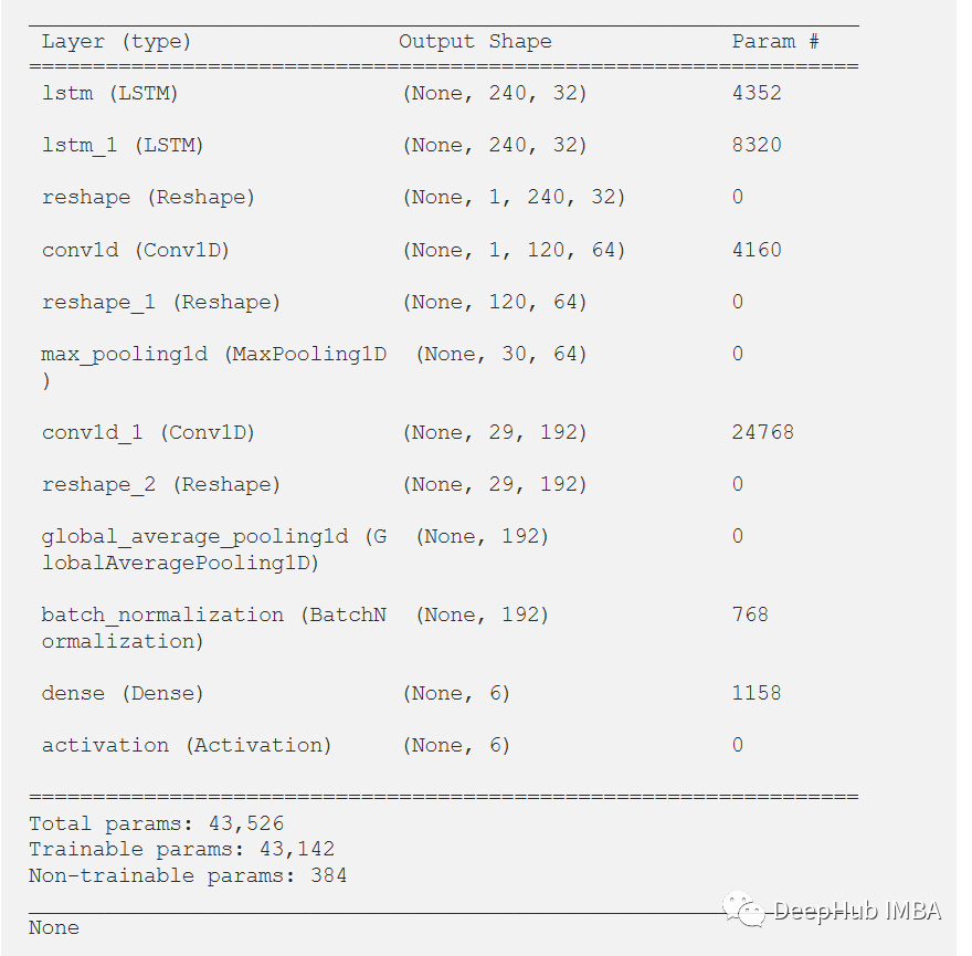
我们使用的模型是一个由8层组成的序列模型。模型前两层由LSTM组成,每个LSTM具有32个神经元,使用的激活函数为Relu。然后是用于提取空间特征的卷积层。
在两层的连接处需要改变LSTM输出维度,因为输出具有3个维度(样本数,时间步长,输入维度),而CNN则需要4维输入(样本数,1,时间步长,输入)。
第一个CNN层具有64个神经元,另一个神经元有128个神经元。在第一和第二CNN层之间,我们有一个最大池层来执行下采样操作。然后是全局平均池(GAP)层将多D特征映射转换为1-D特征向量,因为在此层中不需要参数,所以会减少全局模型参数。然后是BN层,该层有助于模型的收敛性。
最后一层是模型的输出层,该输出层只是具有SoftMax分类器层的6个神经元的完全连接的层,该层表示当前类的概率。
model = Sequential()
model.add(LSTM(32, return_sequences=True, input_shape=(input_shape,1), activation='relu'))
model.add(LSTM(32,return_sequences=True, activation='relu'))
model.add(Reshape((1, 240, 32)))
model.add(Conv1D(filters=64,kernel_size=2, activation='relu', strides=2))
model.add(Reshape((120, 64)))
model.add(MaxPool1D(pool_size=4, padding='same'))
model.add(Conv1D(filters=192, kernel_size=2, activation='relu', strides=1))
model.add(Reshape((29, 192)))
model.add(GlobalAveragePooling1D())
model.add(BatchNormalization(epsilon=1e-06))
model.add(Dense(6))
model.add(Activation('softmax'))

print(model.summary())
训练和结果
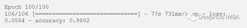
经过训练,模型给出了98.02%的准确率和0.0058的损失。训练F1得分为0.96。
model.compile(loss='categorical_crossentropy', optimizer='adam', metrics=['accuracy'])
history = model.fit(x_train,
                    y_train_hot,
                    batch_size= 192,
                    epochs=100
                   )
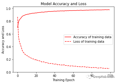
可视化训练的准确性和损失变化图。
plt.figure(figsize=(6, 4))
plt.plot(history.history['accuracy'], 'r', label='Accuracy of training data')
plt.plot(history.history['loss'], 'r--', label='Loss of training data')
plt.title('Model Accuracy and Loss')
plt.ylabel('Accuracy and Loss')
plt.xlabel('Training Epoch')
plt.ylim(0)
plt.legend()
plt.show()
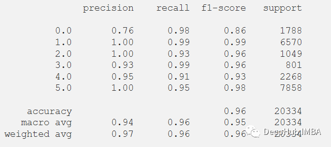
y_pred_train = model.predict(x_train)
max_y_pred_train = np.argmax(y_pred_train, axis=1)
print(classification_report(y_train, max_y_pred_train))
在测试数据集上测试它,但在通过测试集之前,需要对测试集进行相同的预处理。
df_test['X'] = (df_test['X']-df_test['X'].min())/(df_test['X'].max()-df_test['X'].min())
df_test['Y'] = (df_test['Y']-df_test['Y'].min())/(df_test['Y'].max()-df_test['Y'].min())
df_test['Z'] = (df_test['Z']-df_test['Z'].min())/(df_test['Z'].max()-df_test['Z'].min())
x_test, y_test = segments(df_test,
                         TIME_PERIOD,
                         STEP_DISTANCE,
                         LABEL)

x_test = x_test.reshape(x_test.shape[0], input_shape)
x_test = x_test.astype('float32')
y_test = y_test.astype('float32')
y_test = to_categorical(y_test, num_classes)
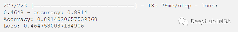
在评估我们的测试数据集后,得到了89.14%的准确率和0.4647的损失。F1测试得分为0.89。
score = model.evaluate(x_test, y_test)
print("Accuracy:", score[1])
print("Loss:", score[0])
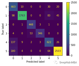
下面绘制混淆矩阵更好地理解对测试数据集的预测。
predictions = model.predict(x_test)
predictions = np.argmax(predictions, axis=1)
y_test_pred = np.argmax(y_test, axis=1)
cm = confusion_matrix(y_test_pred, predictions)
cm_disp = ConfusionMatrixDisplay(confusion_matrix= cm)
cm_disp.plot()
plt.show()
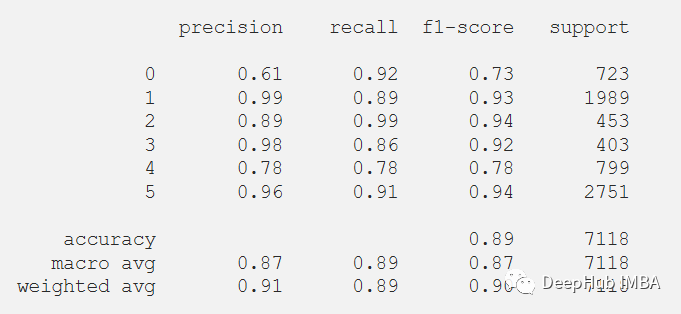
还可以在测试数据集上评估的模型的分类报告。
print(classification_report(y_test_pred, predictions))
总结
LSTM-CNN模型的性能比任何其他机器学习模型要好得多。本文的代码可以在GitHub上找到。
https://github.com/Tanny1810/Human-Activity-Recognition-LSTM-CNN
您可以尝试自己实现它,通过优化模型来提高F1分数。
另:这个模型是来自于Xia Kun, Huang Jianguang, and Hanyu Wang在IEEE期刊上发表的论文LSTM-CNN Architecture for Human Activity Recognition。https://ieeexplore.ieee.org/abstract/document/9043535
作者:Tanmay chauhan