基于图的神经网络是强大的模型,可以学习网络中的复杂模式。在本文中,我们将介绍如何为同构图数据构造PyTorch Data对象,然后训练不同类型的神经网络来预测节点所属的类。这种类型的预测问题通常被称为节点分类。

我们将使用来自Benedek Rozemberczki, Carl Allen和Rik Sarkar于2019年发布的“Multi-scale Attributed Node Embedding”论文中的Facebook Large Page-Page Network¹数据集。
该数据集包含22,470个Facebook页面,按主题分为四类。由不同大小的特征向量表示。数据集还包含Facebook pages 上跟随其他page的信息。网络中有171,992个链接或边。
数据集
第一步是从URL下载数据集。如果手动下载也是可以的,我们这里是为了方便演示
wget https://snap.stanford.edu/data/facebook_large.zip
解压后的数据集包含三个独立的文件:
musae_facebook_edges.csv:该文件包含具有两列的Facebook页面之间的连接图,表示id_1和id_2列是相互连接的,最直接的说法就是图的边。
musae_facebook_target.csv:该文件包含数据集中22,470个Facebook Page的描述和类型。我们试图预测的标签是page_type列,这是一个多类标签,它将每个Facebook页面分为四个类之一,这就是我们图数据的节点。
musae_facebook_features.json:这个文件包含每个Facebook Page的特征向量。键是上面文件的节点id,值是特征向量。
创建PyTorch同构数据对象
为了在PyTorch中训练神经网络,我们必须创建一个数据对象。由于我们的数据集包含相同类型的所有节点,我们将创建一个描述同构图的数据对象。
说明:如果数据集包含多种类型的节点或边,则需要创建一个描述异构图的HeteroData数据对象。
第一步是使用pandas读取CSV文件中的节点数据作然后从json文件中提取特征
但是我们导入JSON文件后发现特征向量大小不一致,嵌入的大小从3到31个不等。
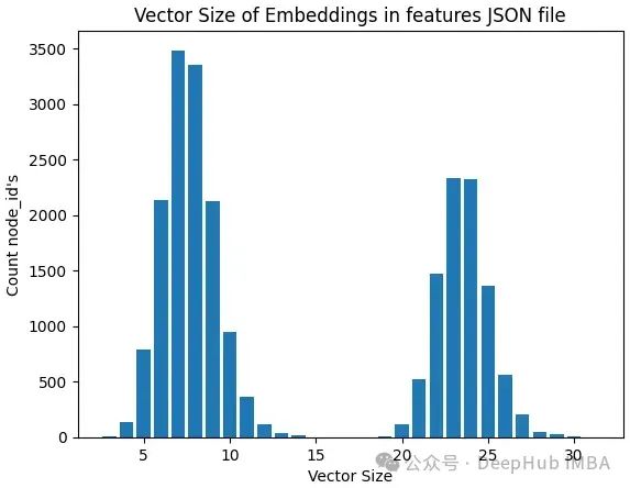
一半情况下模型都期望节点属性或特征具有一致的大小,因此我们需要一些特征转操作。我们将从节点特征中创建张量。由于嵌入的最大大小是31,所以以最大值为例
如果一个节点的特征小于31,将用值0填充剩余的元素。然后,对每个节点的特征进行归一化。下面是所有的代码:
 from torch.nn.utils.rnn import pad_sequence

 def load_node_csv(path, index_col, **kwargs):
   df = pd.read_csv(path, **kwargs)
   mapping = {i: node_id for i, node_id in enumerate(df[index_col].unique())}

   # Load node features
   with open(os.path.join(data_dir, "musae_facebook_features.json"), "r") as json_file:
     features_data = json.load(json_file)

   xs = []
   for index, node_id in mapping.items():
     features = features_data.get(str(index), [])
     if features:
       # Create tensor from feature vector
       features_tensor = torch.tensor(features, dtype=torch.float)
       xs.append(features_tensor)
     else:
       xs.append(torch.zeros(1, dtype=torch.float))

   # Pad features to have vectors of the same size
   padded_features = pad_sequence([torch.tensor(seq) for seq in xs], batch_first=True, padding_value=0)
   mask = padded_features != 0 # mask to indicate which features were padded

   # Create tensor of normaized features for nodes
   mean = torch.mean(padded_features[mask].float())
   std = torch.std(padded_features[mask].float())

   x = (padded_features - mean) / (std + 1e-8)  # final x tensor with normalized features

   return x

 x = load_node_csv(path=os.path.join(data_dir, "musae_facebook_target.csv"), index_col="facebook_id")
上面创建了包含22,470个Facebook Page的特征向量的张量x。
下面就是加载边的数据,也就是建立节点直接的连接
 def load_edge_csv(path, src_index_col, dst_index_col, **kwargs):
   df = pd.read_csv(path, **kwargs)

   src = df[src_index_col].values
   dst = df[dst_index_col].values
   edge_index = torch.tensor([src, dst])

   return edge_index

 edge_index = load_edge_csv(path=os.path.join(data_dir, "musae_facebook_edges.csv"), src_index_col="id_1", dst_index_col="id_2")
得到了一个长度为2的PyTorch张量,一个用于源节点,另一个用于目标节点,总计171,002条边。
清理完数据并将其转换为正确的类型后,我们现在可以为同构图创建PyTorch data对象了:
 # Create homogeneous graph using PyTorch's Data object
 data = Data(x=x, edge_index=edge_index, y=y)
结果数据对象包含22,470个节点,每个节点由大小为31的特征向量表示,在删除重复项和自循环后,节点之间有171,002条边:
>>> Data(x=[22470, 31], edge_index=[2, 171002], y=[22470])
分割数据
为了训练和验证,数据集被分成70%用于训练和30%用于测试,前15,728个节点用于训练,最后6,742个节点用于测试集。
 # Calculate no. of train nodes
 num_nodes = data.num_nodes
 train_percentage = 0.7
 num_train_nodes = int(train_percentage * num_nodes)

 # Create a boolean mask for train mask
 train_mask = torch.zeros(num_nodes, dtype=torch.bool)
 train_mask[: num_train_nodes] = True

 # Add train mask to data object
 data.train_mask = train_mask

 # Create a boolean mask for test mask
 test_mask = ~data.train_mask
 data.test_mask = test_mask
我们使用mask来标识训练和验证集
 >>> Data(
   x=[22470, 31],
   edge_index=[2, 171002],
   y=[22470],
   num_classes=4,
   train_mask=[22470],
   test_mask=[22470]
 )
训练神经网络
我们现在已经可以训练模型了。下面将训练两种不同类型的神经网络,并对它们进行比较。
在训练模型之前我们可以先可视化节点是什么样的
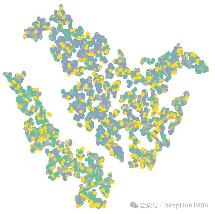
在上面的图表中,似乎有两个大团,但类别区分并不明显。
1、多层感知网络(MLP)
作为对比,我们先训练一个最基础的mlp看看表现
 from torch.nn import Linear
 import torch.nn.functional as F

 class MLP(torch.nn.Module):
   def __init__(self):
     super().__init__()
     torch.manual_seed(123)
     self.lin1 = Linear(data.num_features, 32)
     self.lin2 = Linear(32, 32)
     self.lin3 = Linear(32, 16)
     self.lin4 = Linear(16, 8)
     self.lin5 = Linear(8, data.num_classes)

   def forward(self, x):
     x = self.lin1(x)
     x = F.relu(x)
     x = self.lin2(x)
     x = F.relu(x)
     x = self.lin3(x)
     x = F.relu(x)
     x = self.lin4(x)
     x = F.relu(x)
     x = self.lin5(x)
     x = torch.softmax(x, dim=1)

     return x
创建对象
 class_weights = torch.tensor([1 / i for i in df_agg_classes["proportion"].values], dtype=torch.float)
 model = MLP()
 criterion = torch.nn.CrossEntropyLoss(weight=class_weights)
 optimizer = torch.optim.Adam(model.parameters(), lr=0.01, weight_decay=5e-4)
最终的结构如下:
 >>> MLP(
   (lin1): Linear(in_features=31, out_features=32, bias=True)
   (lin2): Linear(in_features=32, out_features=32, bias=True)
   (lin3): Linear(in_features=32, out_features=16, bias=True)
   (lin4): Linear(in_features=16, out_features=8, bias=True)
   (lin5): Linear(in_features=8, out_features=4, bias=True)
 )
训练循环:
 def train():
   model.train()
   optimizer.zero_grad()  # Clear gradients
   out = model(data.x)  # Perform a single forward pass
   loss = criterion(out[data.train_mask], data.y[data.train_mask])  # Compute loss from training data
   loss.backward()  # Derive gradients
   optimizer.step()  # Update parameters
   return loss
我们训练1000个epoch
 for epoch in range(1, 1001):
   loss = train()
   print(f"Epoch: {epoch:03d}, loss: {loss:.4f}")
然后是验证代码:
 def test():
   model.eval()
   out = model(data.x)
   pred = out.argmax(dim=1)  # Select class with the highest probability
   test_correct = pred[data.test_mask] == data.y[data.test_mask]  # Compare to ground truth labels
   test_acc = int(test_correct.sum()) / int(data.test_mask.sum())  # Calculate fraction of correct predictions
   return test_acc
在测试集上,MLP模型的准确率得分为0.4562,因此该模型能够正确分类46%的节点。
我们可以通过使用TSNE将预测转换为二维并绘制出来,从而将其可视化:
 def visualize(h, color):
   z = TSNE(n_components=2).fit_transform(h.detach().cpu().numpy())
   plt.figure(figsize=(10, 10))
   plt.xticks([])  # create an empty x axis
   plt.yticks([])  # create an empty y axis
   plt.scatter(z[:, 0], z[:, 1], s=70, c=color, cmap="Set2")
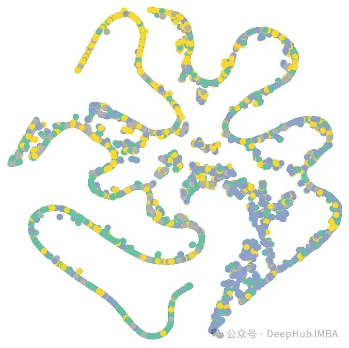
可以看到用MLP模型预测的类别之间没有明显的分离。这里的MLP模型是基于特征向量进行训练的,并且不包含节点之间链接的任何信息。
2、图卷积网络(GCN)
让我们看看如果我们保持大多数参数相同,训练一个图卷积网络(GCN)模型。
 from torch_geometric.nn import GCNConv

 class GCN(torch.nn.Module):
   def __init__(self):
     super().__init__()
     torch.manual_seed(123)
     self.conv1 = GCNConv(data.num_features, 32)
     self.conv2 = GCNConv(32, 32)
     self.conv3 = GCNConv(32, 16)
     self.conv4 = GCNConv(16, 8)
     self.conv5 = GCNConv(8, data.num_classes)

   def forward(self, x, edge_index):
     x = self.conv1(x, edge_index)
     x = F.relu(x)
     x = self.conv2(x, edge_index)
     x = F.relu(x)
     x = self.conv3(x, edge_index)
     x = F.relu(x)
     x = self.conv4(x, edge_index)
     x = F.relu(x)
     x = self.conv5(x, edge_index)
     x = F.log_softmax(x, dim=1)
     return x
剩下的代码基本类似
 model = GCN()
 criterion = torch.nn.CrossEntropyLoss(weight=class_weights)
 optimizer = torch.optim.Adam(model.parameters(), lr=0.01, weight_decay=5e-4)

 def train():
   model.train()
   optimizer.zero_grad()  # Clear gradients
   out = model(data.x, data.edge_index)  # Perform a single forward pass
   loss = criterion(out[data.train_mask], data.y[data.train_mask])  # Compute losses from training data
   loss.backward()  # Derive gradients
   optimizer.step()  # Update parameters
   return loss

 for epoch in range(1, 1001):
   loss = train()
   print(f"Epoch: {epoch:03d}, Loss: {loss:.4f}")
模型验证
 def test():
   model.eval()
   out = model(data.x, data.edge_index)  # Pass in features and edges
   pred = out.argmax(dim=1)  # Get predicted class
   test_correct = pred[data.test_mask] == data.y[data.test_mask]  # Count correct predictions
   test_acc = int(test_correct.sum()) / int(data.test_mask.sum())  # Get proportion of correct predictions
   return test_acc
GCN模型能对测试集中80%的节点进行正确分类!让我们把它画出来: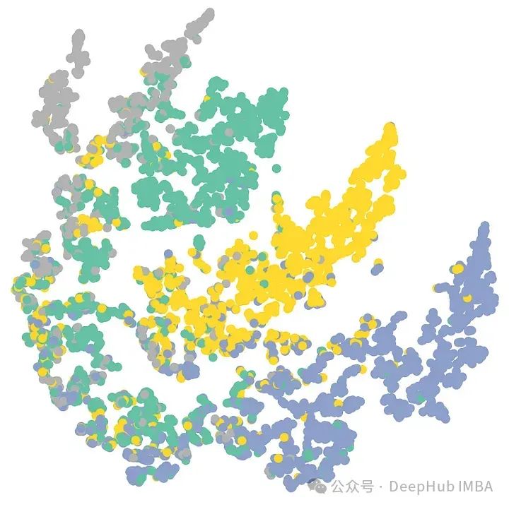
可以看到显示了很好的颜色/类别分离,特别是在图表的中心到右边。这表明带有特征和边缘数据的GCN模型能够较好地对节点进行分类。
总结
在本文中,我们将一个CSV文件转换为数据对象,然后使用PyTorch为节点分类任务构建基于图的神经网络。并且训练了两种不同类型的神经网络——多层感知器(MLP)和图卷积网络(GCN)。结果表明,GCN模型在该数据集上的表现明显优于MLP模型。
本文介绍的主要流程是我们训练图神经网络的基本流程,尤其是前期的数据处理和加载,通过扩展本文的基本流程可以应对几乎所有图神经网络问题。
作者:Claudia Ng