
图结构在现实世界中随处可见。道路、社交网络、分子结构都可以使用图来表示。图是我们拥有的最重要的数据结构之一。
今天有很多的资源可以教我们将机器学习应用于此类数据所需的一切知识。
已经有很多学习有关图机器学习的相关理论和材料,特别是图神经网络,所以本文将避免在这里解释这些内容。如果你对该方面不太熟悉,推荐先看下CS224W,这会对你的入门有很大的帮助。
本篇文章使用PyTorch Geometric来实现我们需要的模型,所以首先就是安装
try:
    # Check if PyTorch Geometric is installed:
    import torch_geometric
except ImportError:
    # If PyTorch Geometric is not installed, install it.
    %pip install -q torch-scatter -f https://pytorch-geometric.com/whl/torch-1.7.0+cu101.html
    %pip install -q torch-sparse -f https://pytorch-geometric.com/whl/torch-1.7.0+cu101.html
    %pip install -q torch-geometric
安装完成后导入我们需要的包
from typing import Callable, List, Optional, Tuple

import matplotlib.pyplot as plt
import numpy as np
import torch
import torch.nn.functional as F
import torch_geometric.transforms as T
from torch import Tensor
from torch.optim import Optimizer
from torch_geometric.data import Data
from torch_geometric.datasets import Planetoid
from torch_geometric.nn import GCNConv
from torch_geometric.utils import accuracy
from typing_extensions import Literal, TypedDict
Cora 数据集
Cora 数据集包含 2708 篇科学出版物,分为七类之一。引用的网络由 5429 个链接组成。数据集中的每个出版物都由一个 0/1 值的词向量描述,该向量表示字典中对应单词是否存在。该词典包含1433个独特的单词。
首先让我们探索这个数据集以了解它是如何生成的:
dataset = Planetoid("/tmp/Cora", name="Cora")
num_nodes = dataset.data.num_nodes
# For num. edges see:
# - https://github.com/pyg-team/pytorch_geometric/issues/343
# - https://github.com/pyg-team/pytorch_geometric/issues/852
num_edges = dataset.data.num_edges // 2
train_len = dataset[0].train_mask.sum()
val_len = dataset[0].val_mask.sum()
test_len = dataset[0].test_mask.sum()
other_len = num_nodes - train_len - val_len - test_len
print(f"Dataset: {dataset.name}")
print(f"Num. nodes: {num_nodes} (train={train_len}, val={val_len}, test={test_len}, other={other_len})")
print(f"Num. edges: {num_edges}")
print(f"Num. node features: {dataset.num_node_features}")
print(f"Num. classes: {dataset.num_classes}")
print(f"Dataset len.: {dataset.len()}")
输出
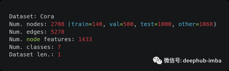
我们可以看到一些信息:
- 为了获得正确的边数,我们必须将数据属性“num_edges”除以2,这是因为 Pytorch Geometric “将每个链接保存为两个方向的无向边”。
- 这样做以后数字也对不上,显然是因为“Cora 数据集有重复的边”,需要我们进行数据的清洗
- 另一个奇怪的事实是,移除用于训练、验证和测试的节点后,还有其他节点。
- 最后就是我们可以看到Cora数据集实际上只包含一个图。
我们使用 Glorot & Bengio (2010) 中描述的初始化来初始化权重,并相应地(行)归一化输入特征向量。( Kipf & Welling ICLR 2017 arxiv:1609.02907)
Glorot 初始化默认由 PyTorch Geometric 完成,行的归一化目的是使每个节点的特征总和为 1,所以我们必须显式的进行处理:
dataset = Planetoid("/tmp/Cora", name="Cora")
print(f"Sum of row values without normalization: {dataset[0].x.sum(dim=-1)}")

dataset = Planetoid("/tmp/Cora", name="Cora", transform=T.NormalizeFeatures())
print(f"Sum of row values with normalization: {dataset[0].x.sum(dim=-1)}")
输出如下:

图卷积网络GCN
现在我们有了数据,是时候定义我们的图卷积网络(GCN)了!
class GCN(torch.nn.Module):
    def __init__(
        self,
        num_node_features: int,
        num_classes: int,
        hidden_dim: int = 16,
        dropout_rate: float = 0.5,
    ) -> None:
        super().__init__()
        self.dropout1 = torch.nn.Dropout(dropout_rate)
        self.conv1 = GCNConv(num_node_features, hidden_dim)
        self.relu = torch.nn.ReLU(inplace=True)
        self.dropout2 = torch.nn.Dropout(dropout_rate)
        self.conv2 = GCNConv(hidden_dim, num_classes)

    def forward(self, x: Tensor, edge_index: Tensor) -> torch.Tensor:
        x = self.dropout1(x)
        x = self.conv1(x, edge_index)
        x = self.relu(x)
        x = self.dropout2(x)
        x = self.conv2(x, edge_index)
        return x
print("Graph Convolutional Network (GCN):")
GCN(dataset.num_node_features, dataset.num_classes)
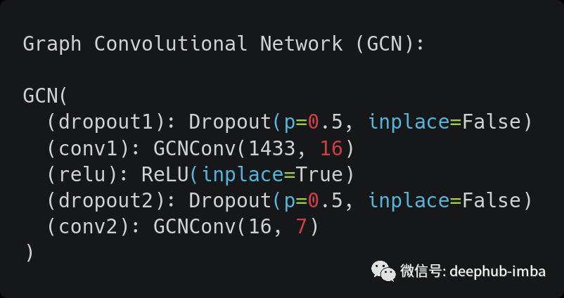
如果查看了 PyTorch Geometric 文档中的实现,甚至是 Thomas Kipf 在该框架中的实现,就会发现有一些不一致的地方(例如有两个 dropout 层)。实际上这是因为这两个都不完全与 TensorFlow 中的原始实现相同,所以我们这里不考虑原始实现,只使用PyTorch Geometric提供的模型。
训练和评估
在训练之前,我们准备训练和评估步骤:
LossFn = Callable[[Tensor, Tensor], Tensor]
Stage = Literal["train", "val", "test"]

def train_step(
    model: torch.nn.Module, data: Data, optimizer: torch.optim.Optimizer, loss_fn: LossFn
) -> Tuple[float, float]:
    model.train()
    optimizer.zero_grad()
    mask = data.train_mask
    logits = model(data.x, data.edge_index)[mask]
    preds = logits.argmax(dim=1)
    y = data.y[mask]
    loss = loss_fn(logits, y)
    # + L2 regularization to the first layer only
    # for name, params in model.state_dict().items():
    #     if name.startswith("conv1"):
    #         loss += 5e-4 * params.square().sum() / 2.0

    acc = accuracy(preds, y)
    loss.backward()
    optimizer.step()
    return loss.item(), acc

@torch.no_grad()
def eval_step(model: torch.nn.Module, data: Data, loss_fn: LossFn, stage: Stage) -> Tuple[float, float]:
    model.eval()
    mask = getattr(data, f"{stage}_mask")
    logits = model(data.x, data.edge_index)[mask]
    preds = logits.argmax(dim=1)
    y = data.y[mask]
    loss = loss_fn(logits, y)
    # + L2 regularization to the first layer only
    # for name, params in model.state_dict().items():
    #     if name.startswith("conv1"):
    #         loss += 5e-4 * params.square().sum() / 2.0

    acc = accuracy(preds, y)
    return loss.item(), acc
模型将整个图作为输入,而输出和目标的掩码取决于是训练、验证还是测试。
还是来自 Kipf & Welling(ICLR 2017):我们使用 Adam (Kingma & Ba, 2015) 训练所有模型最多 200 个轮次,学习率为 0.01并使用窗口大小为 10的早停机制,即如果连续 10 个 epoch验证损失没有减少,我们就停止训练 。
这里的一些代码已被注释掉并且未真正使用,这是因为它尝试将 L2 正则化仅应用于原始实现中的第一层。一般情况下使用 PyTorch 无法轻松地 100% 复制在 TensorFlow 中所有的工作,所以在这个例子中,经过测试最好的是使用权重衰减的Adam优化器。
class HistoryDict(TypedDict):
    loss: List[float]
    acc: List[float]
    val_loss: List[float]
    val_acc: List[float]

def train(
    model: torch.nn.Module,
    data: Data,
    optimizer: torch.optim.Optimizer,
    loss_fn: LossFn = torch.nn.CrossEntropyLoss(),
    max_epochs: int = 200,
    early_stopping: int = 10,
    print_interval: int = 20,
    verbose: bool = True,
) -> HistoryDict:
    history = {"loss": [], "val_loss": [], "acc": [], "val_acc": []}
    for epoch in range(max_epochs):
        loss, acc = train_step(model, data, optimizer, loss_fn)
        val_loss, val_acc = eval_step(model, data, loss_fn, "val")
        history["loss"].append(loss)
        history["acc"].append(acc)
        history["val_loss"].append(val_loss)
        history["val_acc"].append(val_acc)
        # The official implementation in TensorFlow is a little different from what is described in the paper...
        if epoch > early_stopping and val_loss > np.mean(history["val_loss"][-(early_stopping + 1) : -1]):
            if verbose:
                print("\nEarly stopping...")

            break

        if verbose and epoch % print_interval == 0:
            print(f"\nEpoch: {epoch}\n----------")
            print(f"Train loss: {loss:.4f} | Train acc: {acc:.4f}")
            print(f"  Val loss: {val_loss:.4f} |   Val acc: {val_acc:.4f}")

    test_loss, test_acc = eval_step(model, data, loss_fn, "test")
    if verbose:
        print(f"\nEpoch: {epoch}\n----------")
        print(f"Train loss: {loss:.4f} | Train acc: {acc:.4f}")
        print(f"  Val loss: {val_loss:.4f} |   Val acc: {val_acc:.4f}")
        print(f" Test loss: {test_loss:.4f} |  Test acc: {test_acc:.4f}")

    return history
def plot_history(history: HistoryDict, title: str, font_size: Optional[int] = 14) -> None:
    plt.suptitle(title, fontsize=font_size)
    ax1 = plt.subplot(121)
    ax1.set_title("Loss")
    ax1.plot(history["loss"], label="train")
    ax1.plot(history["val_loss"], label="val")
    plt.xlabel("Epoch")
    ax1.legend()

    ax2 = plt.subplot(122)
    ax2.set_title("Accuracy")
    ax2.plot(history["acc"], label="train")
    ax2.plot(history["val_acc"], label="val")
    plt.xlabel("Epoch")
    ax2.legend()
需要注意的是,论文中描述早停逻辑与官方实现略有不同:并不是是验证损失不减少比最后十个值的平均值而是当它更大时停止。
下面我们开始训练
SEED = 42
MAX_EPOCHS = 200
LEARNING_RATE = 0.01
WEIGHT_DECAY = 5e-4
EARLY_STOPPING = 10

torch.manual_seed(SEED)
device = torch.device("cuda" if torch.cuda.is_available() else "cpu")

model = GCN(dataset.num_node_features, dataset.num_classes).to(device)
data = dataset[0].to(device)
optimizer = torch.optim.Adam(model.parameters(), lr=LEARNING_RATE, weight_decay=WEIGHT_DECAY)
history = train(model, data, optimizer, max_epochs=MAX_EPOCHS, early_stopping=EARLY_STOPPING)
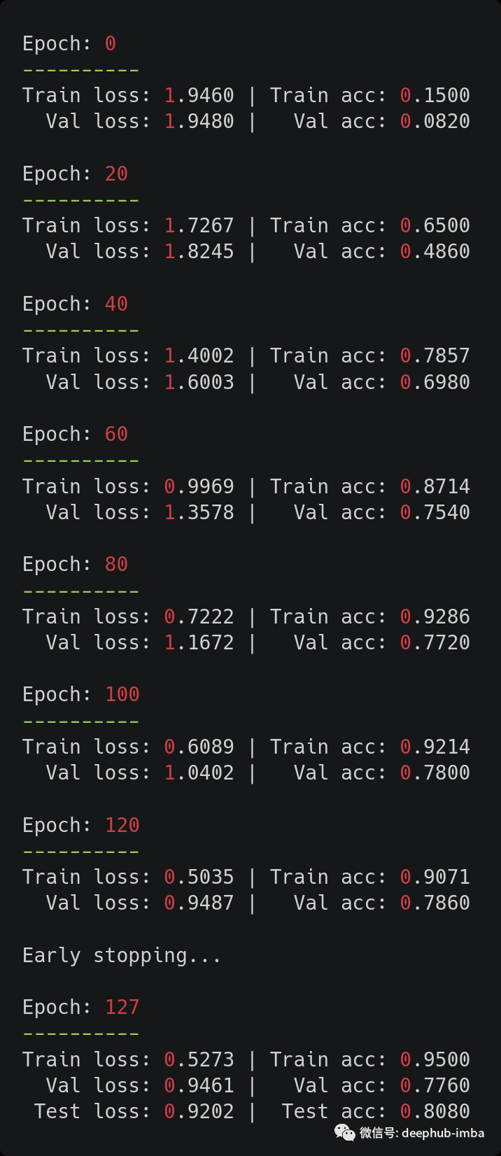
结果还可以,我们获得了与原始论文中报告的一致的测试准确度(论文中为 81.5%)。由于这是一个小数据集,因此这些结果对选择的随机种子很敏感。缓解该问题的一种解决方案是像作者一样取 100(或更多)次运行的平均值。
最后,让我们看一下损失和准确率曲线。
plt.figure(figsize=(12, 4))
plot_history(history, "GCN")
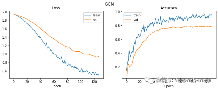
虽然验证损失持续下降了更长的时间,但从第 20 轮开始,验证准确率实际上已经稳定了。
引用
原始论文:
Semi-Supervised Classification with Graph Convolutional Networks :https://arxiv.org/abs/1609.02907
PyG (PyTorch Geometric) 文档:https://pytorch-geometric.readthedocs.io/en/latest/
作者:Mario Namtao Shianti Larcher