
第5章 深度学习用于计算机视觉
本章将介绍卷积神经网络,也叫convnet,它是计算机视觉应用几乎都在使用的一种深度学习模型。
5.1 卷积神经网络简介
实例化一个小型的卷积神经网络:
from keras import layers
from keras import models

model = models.Sequential()
model.add(layers.Conv2D(32, (3, 3), activation='relu', input_shape=(28, 28, 1)))
model.add(layers.MaxPooling2D((2, 2)))
model.add(layers.Conv2D(64, (3, 3), activation='relu'))
model.add(layers.MaxPooling2D((2, 2)))
model.add(layers.Conv2D(64, (3, 3), activaition='relu'))
重要的是,卷积神经网络接收形状为(image_height, image_width, image_channels)的输入张量(不包括批量维度)。我们来看一下目前卷积神经网络的架构:
print(model.summary())
Model: "sequential"
_________________________________________________________________
 Layer (type)                Output Shape              Param #
=================================================================
 conv2d (Conv2D)             (None, 26, 26, 32)        320

 max_pooling2d (MaxPooling2D  (None, 13, 13, 32)       0
 )

 conv2d_1 (Conv2D)           (None, 11, 11, 64)        18496

 max_pooling2d_1 (MaxPooling  (None, 5, 5, 64)         0
 2D)

 conv2d_2 (Conv2D)           (None, 3, 3, 64)          36928

=================================================================
Total params: 55,744
Trainable params: 55,744
Non-trainable params: 0
_________________________________________________________________
None
在卷积神经网络上添加分类器:
model.add(layers.Flatten())
model.add(layers.Dense(64, activation='relu'))
model.add(layers.Dense(10, activation='softmax'))

print(model.summary())
现在的网络架构如下:
Model: "sequential"
_________________________________________________________________
 Layer (type)                Output Shape              Param #
=================================================================
 conv2d (Conv2D)             (None, 26, 26, 32)        320

 max_pooling2d (MaxPooling2D  (None, 13, 13, 32)       0
 )

 conv2d_1 (Conv2D)           (None, 11, 11, 64)        18496

 max_pooling2d_1 (MaxPooling  (None, 5, 5, 64)         0
 2D)

 conv2d_2 (Conv2D)           (None, 3, 3, 64)          36928

 flatten (Flatten)           (None, 576)               0

 dense (Dense)               (None, 64)                36928

 dense_1 (Dense)             (None, 10)                650

=================================================================
Total params: 93,322
Trainable params: 93,322
Non-trainable params: 0
_________________________________________________________________
None
在MNIST图像上训练卷积神经网络:
from keras.datasets import mnist
from keras.utils.np_utils import to_categorical

(train_images, train_labels), (test_images, test_labels) = mnist.load_data()

train_images = train_images.reshape((60000, 28, 28, 1))
train_images = train_images.astype('float32') / 255

test_images = test_images.reshape((10000, 28, 28, 1))
test_images = test_images.astype('float32') / 255

train_labels = to_categorical(train_labels)
test_labels = to_categorical(test_labels)

model.compile(optimizer='rmsprop',
              loss='categorical_crossentropy',
              metrics=['accuracy'])
model.fit(train_images, train_labels, epochs=5, batch_size=64)
完整代码:
from keras.datasets import mnist
from keras.utils.np_utils import to_categorical
from keras import layers
from keras import models

model = models.Sequential()
model.add(layers.Conv2D(32, (3, 3), activation='relu', input_shape=(28, 28, 1)))
model.add(layers.MaxPooling2D((2, 2)))
model.add(layers.Conv2D(64, (3, 3), activation='relu'))
model.add(layers.MaxPooling2D((2, 2)))
model.add(layers.Conv2D(64, (3, 3), activation='relu'))
model.add(layers.Flatten())
model.add(layers.Dense(64, activation='relu'))
model.add(layers.Dense(10, activation='softmax'))

(train_images, train_labels), (test_images, test_labels) = mnist.load_data()

train_images = train_images.reshape((60000, 28, 28, 1))
train_images = train_images.astype('float32') / 255

test_images = test_images.reshape((10000, 28, 28, 1))
test_images = test_images.astype('float32') / 255

train_labels = to_categorical(train_labels)
test_labels = to_categorical(test_labels)

model.compile(optimizer='rmsprop',
              loss='categorical_crossentropy',
              metrics=['accuracy'])
model.fit(train_images, train_labels, epochs=5, batch_size=64)

test_loss, test_acc = model.evaluate(test_images, test_labels)

print(test_acc)
Epoch 1/5
938/938 [==============================] - 33s 24ms/step - loss: 0.1748 - accuracy: 0.9453
Epoch 2/5
938/938 [==============================] - 26s 28ms/step - loss: 0.0481 - accuracy: 0.9848
Epoch 3/5
938/938 [==============================] - 21s 22ms/step - loss: 0.0331 - accuracy: 0.9895
Epoch 4/5
938/938 [==============================] - 21s 22ms/step - loss: 0.0250 - accuracy: 0.9926
Epoch 5/5
938/938 [==============================] - 20s 22ms/step - loss: 0.0191 - accuracy: 0.9940
313/313 [==============================] - 4s 9ms/step - loss: 0.0348 - accuracy: 0.9898
0.989799976348877
5.1.1 卷积运算
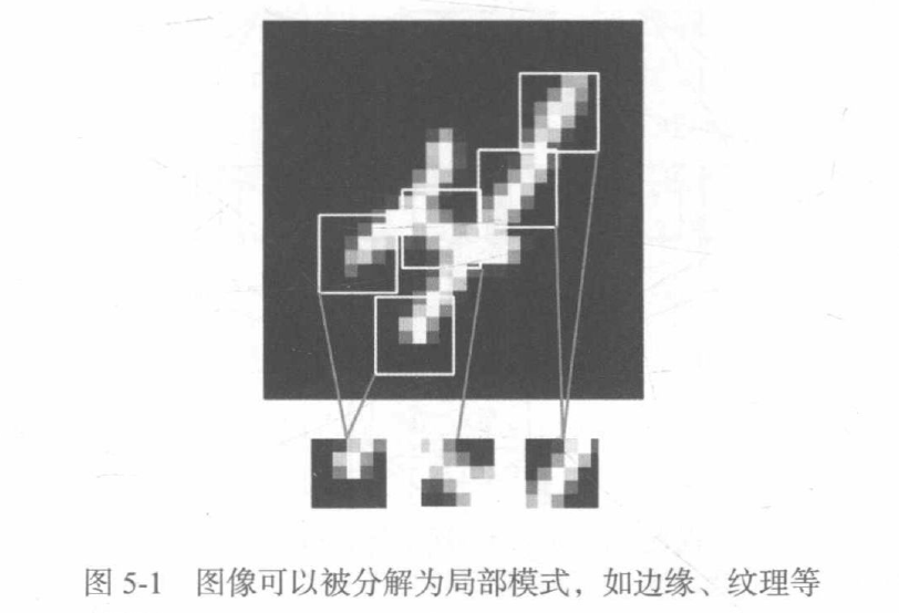
密集连接层和圈进层的根本区别在于,Dense层从输入特征空间学到的是全局模式(比如对于MNIST数字,全局模式就是涉及所有像素的模式),而卷积层学到的是局部模式,对于图像来说,学到的就是在输入图像的二维小窗口中发现的模式。
这个重要特性使卷积神经网络具有以下两个有趣的性质:
1.卷积神经网络学到的模式具有平移不变性。卷积神经网络在图像右下角学到某个模式之后,它可以在任何地方识别这个模式,比如左上角。对于密集连接网络来说,如果模式出现在新的位置,它只能重新学习这个模式。这使得卷积神经网络在处理图像时可以高效利用数据(因为视觉世界从根本上具有平移不变性),它只需要更少的训练样本就可以学到具有泛化能力的数据表示。
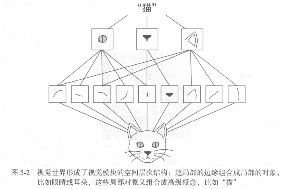
2.卷积神经网络可以学到模式的空间层次结构。第一个卷积层将学习较小的局部模式(比如边缘),第二个卷积层将学习由第一层特征组成的更大的模式,以此类推。这使得卷积神经网络可以有效地学习越来越复杂、越来越抽象的视觉概念(因为视觉世界从根本上具有空间层次结构)。
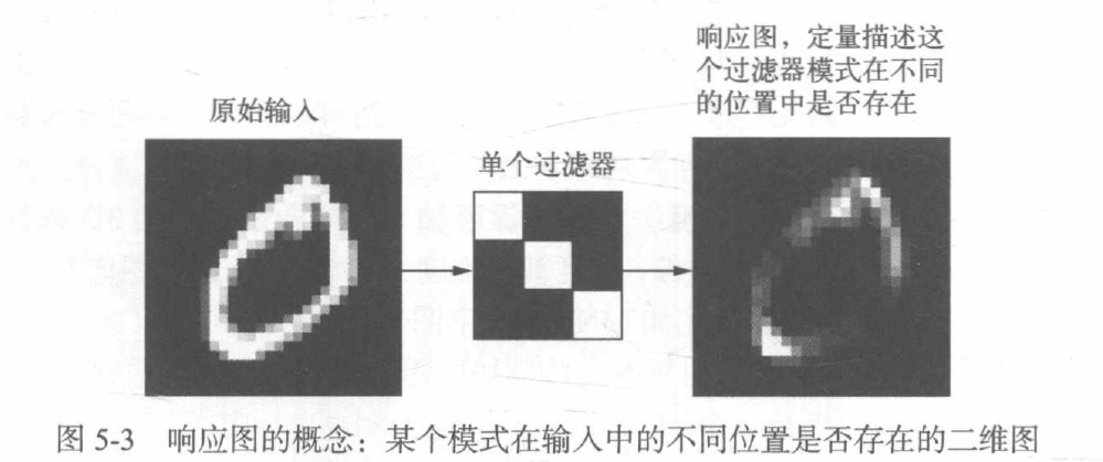
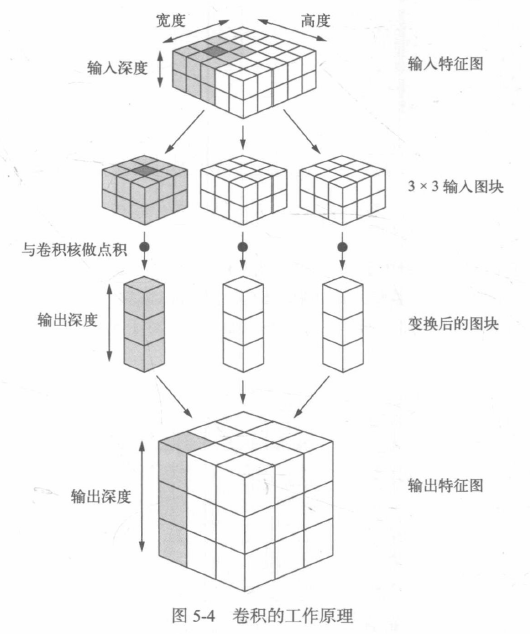
对于包含两个空间轴(高度和宽度)和一个深度轴(也叫通道轴)的3D张量,其卷积也叫特征图。对于RGB图像,深度轴的维度大小等于3, 因为图像有3个颜色通道:红色、绿色和蓝色。对于黑白图像(比如MNIST数字图像),深度等于1(表示灰度等级)。卷积运算从输入特征图中提取图块,并对所有这些图块应用相同的变换,生成输出特征图。该输出特征图仍是一个3D张量,具有宽度和高度,其深度可以任意取值,因为输出深度是层的参数,深度轴的不同通道不再像RGB那样代表特定颜色,而是代表过滤器,过滤器对输入数据的某一方面进行编码 。
特征图:深度轴的每个维度都是一个特征(或过滤器),而2D张量output[:, :, n]是这个过滤器在输入上的响应的二维空间图。
卷积由以下两个关键参数所定义。
1.从输入中提取的图块尺寸。
2.输出特征图的深度:卷积所计算的过滤器的数量。
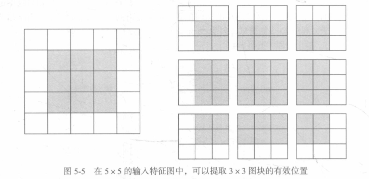
卷积的工作原理:在3D输入特征图上滑动这些3x3或5x5的窗口,在每个可能的位置停止并提取周围特征的3D图块[形状为(window_height, window_width, input_depth)]。然后每个3D图块与学到的同一个权重矩阵[叫作卷积核]做张量积,转换成形状为(output_depth,)的1D向量。然后对所有这些向量进行空间重组,使其转换为形状为(height, width, output_depth)的3D输出特征图。输出特征图中的每个空间位置都对应于输入特征图中的相同位置。
输出的宽度和高度可能与输入的宽度和高度不同,不同的原因可能有两点:
(1)边界效应,可以通过对输入特征图进行填充来抵消;
(2)使用了步幅。
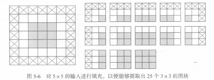
** 1.理解边界效应与填充**
如果你希望输出特征图的空间维度与输入相同,那么可以使用填充。填充是在输入特征图的每一边添加适当数据的行和列,使得每个输入方块都能作为卷积窗口的中心。
**2.理解卷积步幅 **
影响输出尺寸的另一个因素是步幅的概念。目前为止,对卷积的描述都假设卷积窗口的中心方块都是相邻的。但两个连续窗口的距离是卷积的一个参数,叫作步幅,默认值为1,也可以使用步进卷积,即步幅大于1的卷积。
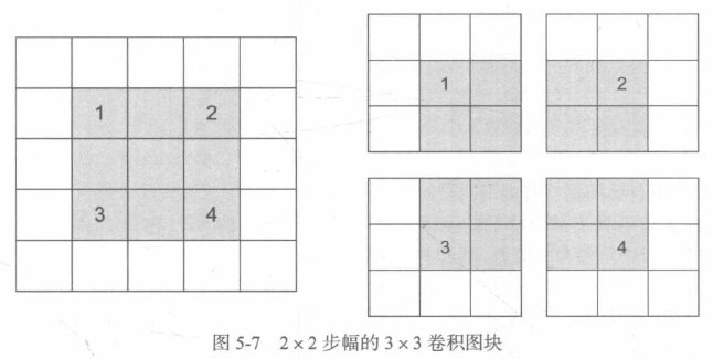
步幅为2意味着特征图的宽度和高度都被做了2倍下采样(除了边界效应引起的变化)。虽然步进卷积对某些类型的模型可能有用,但在实践中很少使用。
为了对特征图进行下采样,我们不用步幅,而是通常使用最大池化运算。
5.1.2 最大池化运算
在卷积神经网络示例中,你可能注意到,在每个MaxPooling2D层之后,特征图的尺寸都会减半。例如,在第一个MaxPooling2D层之前,特征图的尺寸是26x26,但最大池化运算将其减半为13x13。这就是最大池化的作用:对特征图进行下采样,与步进卷积类似。
最大池化是从输入特征图中提取窗口,并输出每个通道的最大值,它使用硬编码的max张量运算对局部图块进行变换,而不是使用学到的线性变换。最大池化与卷积的最大不同之处在于,最大池化通常使用2x2的窗口和步幅2,其目的是将特征图下采样2倍。与此相对的是,卷积通常使用3x3窗口和步幅1。
from keras import layers
from keras import models

model_no_max_pool = models.Sequential()
model_no_max_pool.add(layers.Conv2D(32, (3, 3), activation='relu', input_shape=(28, 28, 1)))
model_no_max_pool.add(layers.Conv2D(64, (3, 3), activation='relu'))
model_no_max_pool.add(layers.Conv2D(64, (3, 3), activation='relu'))

print(model_no_max_pool.summary())
Model: "sequential"
_________________________________________________________________
 Layer (type)                Output Shape              Param #
=================================================================
 conv2d (Conv2D)             (None, 26, 26, 32)        320

 conv2d_1 (Conv2D)           (None, 24, 24, 64)        18496

 conv2d_2 (Conv2D)           (None, 22, 22, 64)        36928

=================================================================
Total params: 55,744
Trainable params: 55,744
Non-trainable params: 0
_________________________________________________________________
None

正在上传…重新上传取消正在上传…重新上传取消
这种架构有如下两点问题:
1.这种架构不利于学习特征的空间层级结构。
2.最后一层的特征图对每个样本共有22x22x64=30976个元素。这太多了,如果你将其展平并在上面添加一个大小为512的Dense层,那一层将会有1580万个参数。这对于这样一个小模型来说太多了,会导致严重的过拟合。
简而言之,使用下采样的原因,一是减少需要处理的特征图的元素个数,二是通过让连续的卷积层的观察窗口越来越大(即窗口覆盖原始输入的比例越来越大),从而引入空间过滤器的层级结构。
最大池化不是实现这种下采样的唯一方法,还可以在前一个卷积层中使用步幅来实现。此外,还可以使用平均池化来代替最大池化,其方法是将每个局部输入图块变换为取该图块各通道的平均值,而不是最大值。但最大池化的效果往往比这些替代方法更好。
简而言之,原因在于特征中往往编码了某种模式或概念在特征图的不同位置是否存在(因此得名特征图),而观察不同特征的最大值而不是平均值能够给出更多的信息。因此,最合理的子采样策略是首先生成密集的特征图(通过步进卷积)或对输入图块取平均,因为后两种方法可能导致错过或淡化特征是否存在的信息。
5.2 在小型数据集上从头开始训练一个卷积神经网络
5.2.1 深度学习与小数据问题的相关性
深度学习的一个基本特性就是能够独立地在训练数据中找到有趣的特征,无须人为的特征工程,而这只有拥有大量训练样本时才能实现,对于输入样本的维度非常高(比如图像)的问题尤其如此。
由于卷积神经网络学到的是局部的、平移不变的特征,它对于感知问题可以高效地利用数据。虽然数据相对较少,但在非常小的图像数据集上从头开始训练一个卷积神经网络,仍然可以得到不错的结果,而且无须任何自定义的特征工程。
此外,深度学习模型本质上具有高度的可复用性,比如,已有一个在大规模数据集上训练的图像分类模型或语音转文本模型,你只需做很小的修改就能将其复用与完全不同的问题。特别是在计算机视觉领域,许多预训练的模型(通常都是在ImageNet数据集上训练得到的)现在都可以公开下载,并可以用于在数据很少的情况下构建强大的视觉模型。
5.2.2 下载数据
将图像复制到训练、验证和测试的目录:
import os
import shutil

original_dataset_dir = r'E:\train\train'

base_dir = r'E:\train\cats_and_dogs_small'
os.mkdir(base_dir)

train_dir = os.path.join(base_dir, 'train')
os.mkdir(train_dir)
validation_dir = os.path.join(base_dir, 'validation')
os.mkdir(validation_dir)
test_dir = os.path.join(base_dir, 'test')
os.mkdir(test_dir)

train_cats_dir = os.path.join(train_dir, 'cats')
os.mkdir(train_cats_dir)

train_dogs_dir = os.path.join(train_dir, 'dogs')
os.mkdir(train_dogs_dir)

validation_cats_dir = os.path.join(validation_dir, 'cats')
os.mkdir(validation_cats_dir)

validation_dogs_dir = os.path.join(validation_dir, 'dogs')
os.mkdir(validation_dogs_dir)

test_cats_dir = os.path.join(test_dir, 'cats')
os.mkdir(test_cats_dir)

test_dogs_dir = os.path.join(test_dir, 'dogs')
os.mkdir(test_dogs_dir)

fnames = ['cat.{}.jpg'.format(i) for i in range(1000)]
for fname in fnames:
    src = os.path.join(original_dataset_dir, fname)
    dst = os.path.join(train_cats_dir, fname)
    shutil.copyfile(src, dst)

fnames = ['cat.{}.jpg'.format(i) for i in range(1000, 1500)]
for fname in fnames:
    src = os.path.join(original_dataset_dir, fname)
    dst = os.path.join(validation_cats_dir, fname)
    shutil.copyfile(src, dst)

fnames = ['cat.{}.jpg'.format(i) for i in range(1500, 2000)]
for fname in fnames:
    src = os.path.join(original_dataset_dir, fname)
    dst = os.path.join(test_cats_dir, fname)
    shutil.copyfile(src, dst)

fnames = ['dog.{}.jpg'.format(i) for i in range(1000)]
for fname in fnames:
    src = os.path.join(original_dataset_dir, fname)
    dst = os.path.join(train_dogs_dir, fname)
    shutil.copyfile(src, dst)

fnames = ['dog.{}.jpg'.format(i) for i in range(1000, 1500)]
for fname in fnames:
    src = os.path.join(original_dataset_dir, fname)
    dst = os.path.join(validation_dogs_dir, fname)
    shutil.copyfile(src, dst)

fnames = ['dog.{}.jpg'.format(i) for i in range(1500, 2000)]
for fname in fnames:
    src = os.path.join(original_dataset_dir, fname)
    dst = os.path.join(test_dogs_dir, fname)
    shutil.copyfile(src, dst)

print('total training cat image:', len(os.listdir(train_cats_dir)))
print('total training dog images:', len(os.listdir(train_dogs_dir)))
print('total validation cat images:', len(os.listdir(validation_cats_dir)))
print('total validation dog images:', len(os.listdir(validation_dogs_dir)))
print('total test cat images:', len(os.listdir(test_cats_dir)))
print('total test cat images:', len(os.listdir(test_dogs_dir)))
total training cat image: 1000
total training dog image: 1000
total validation cat image: 500
total validation dog image: 500
total test cat image: 500
total test dog image: 500
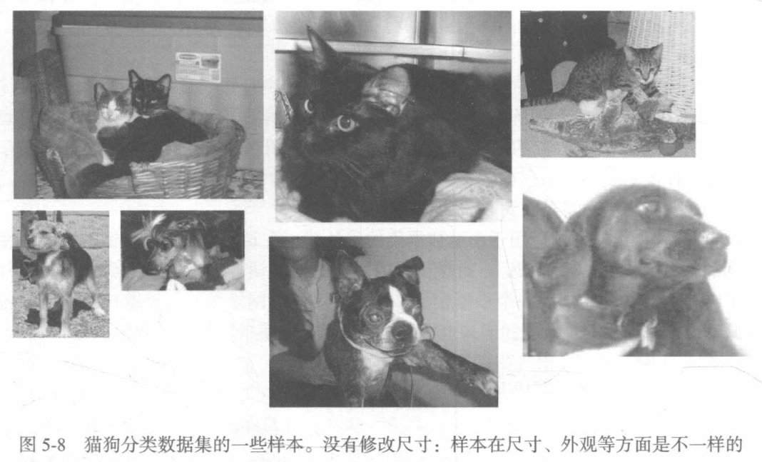
所以我们的确有2000张训练图像、1000张验证图像和1000张测试图像。每个分组中两个类别的样本数相同,这是一个平衡的二分类问题,分类精度可作为衡量成功的指标。
5.2.3 构建网络
你面对的是一个二分类问题,所以网络最后一层是使用sigmoid激活的单一单元(大小为1的Dense层)。这个单元将对某个类别的概率进行编码。
将猫狗分类的小型卷积神经网络实例化:
from keras import layers
from keras import models

model = models.Sequential()
model.add(layers.Conv2D(32, (3, 3), activation='relu', input_shape=(150, 150, 3)))
model.add(layers.MaxPooling2D((2, 2)))
model.add(layers.Conv2D(64, (3, 3), activation='relu'))
model.add(layers.MaxPooling2D((2, 2)))
model.add(layers.Conv2D(128, (3, 3), activation='relu'))
model.add(layers.MaxPooling2D((2, 2)))
model.add(layers.Conv2D(128, (3, 3), activation='relu'))
model.add(layers.MaxPooling2D((2, 2)))
model.add(layers.Flatten())
model.add(layers.Dense(512, activation='relu'))
model.add(layers.Dense(1, activation='sigmoid'))

print(model.summary())
配置模型用于训练:
model.compile(loss='binary_crossentropy',
              optimizer=optimizers.RMSprop(lr=1e-4),
              metrics=['acc'])
5.2.4 数据预处理
现在,数据以JPEG文件的形式形式保存在硬盘中,所以数据预处理步骤大致如下:
(1)读取图像文件;
(2)将JPEG文件解码为RGB像素网格;
(3)将这些像素网络转换为浮点数张量;
(4)将像素值(0~255范围内)缩放到[0, 1]区间(神经网络喜欢处理较小的输入值)。
使用ImageDataGenerator从目录中读取图像:
from keras.preprocessing.image import ImageDataGenerator

train_datagen = ImageDataGenerator(rescale=1./255)
test_datagen = ImageDataGenerator(rescale=1./255)

train_generator = train_datagen.flow_from_directory(
    train_dir,
    target_size=(150, 150),
    batch_size=20,
    class_mode='binary')

validation_generator = test_datagen.flow_from_directory(
    validation_dir,
    target_size=(150, 150),
    batch_size=20,
    class_mode='binary'
)
利用批量生成器拟合模型:
history = model.fit_generator(
    train_generator,
    steps_per_epoch=100,
    epochs=30,
    validation_data=validation_generator,
    validation_steps=50
)
保存模型:
model.save('cats_and_dogs_small_1.h5')
绘制训练过程中的损失曲线和精度曲线:
import matplotlib.pyplot as plt

acc = history.history['acc']
val_acc = history.history['val_acc']
loss = history.history['loss']
val_loss = history.history['val_loss']

epochs = range(1, len(acc) + 1)

plt.plot(epochs, acc, 'bo', label='Training acc')
plt.plot(epochs, val_acc, 'b', label='Validation acc')
plt.title('Training and validation accuracy')
plt.legend()

plt.figure()

plt.plot(epochs, loss, 'bo', label='Training loss')
plt.plot(epochs, val_loss, 'b', label='Validation loss')
plt.title('Training and validation loss')
plt.legend()

plt.show()
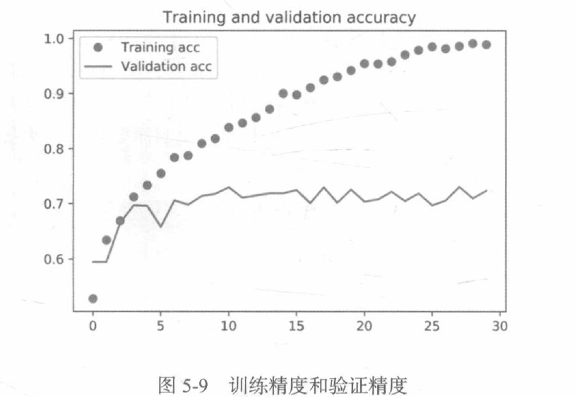
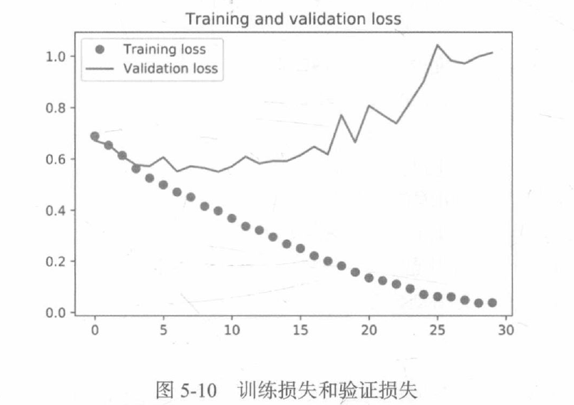
从这些图像中都能看出过拟合的特征。训练精度随着时间线性增加,直到接近100%,而验证精度则停留在70%~72%。验证损失仅在5轮后就达到最小值,然后保持不变,而训练损失则一直线性下降,直到接近于0。因为训练样本相对较少(2000个),所以过拟合是你最关心的问题。
5.2.5 使用数据增强
过拟合的原因是学习样本太少,导致无法训练出能够泛化到新数据的模型。如果拥有无限的数据,那么模型能够观察到数据分布的所有内容,这样就永远不会过拟合。数据增强是从现有的训练样本中生成更多的训练数据,其方法是利用多种能够生成可信图像的随机变换来增加样本。其目标是,模型在训练时不会两次查看完全相同的图像。这让模型能够观察到数据的更多内容,从而具有更好的泛化能力。
利用ImageDataGenerator来设置数据增强:
datagen = ImageDataGenerator(
    rotation_range=40,
    width_shift_range=0.2,
    heigth_shift_range=0.2,
    shear_range=0.2,
    zoom_range=0.2,
    horizontal_flip=True,
    fill_mode='nearest'
)
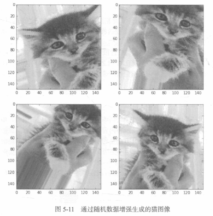
显示几个随机增强后的训练图像:
# 显示几个随机增强后的训练图像
fnames = [os.path.join(train_cats_dir, fname) for fname in os.listdir(train_cats_dir)]
img_path = fnames[3]  # 选择一张图像进行增强
img = image.load_img(img_path, target_size=(150, 150))  # 读取图像并调整大小
x = image.img_to_array(img)  # 将其转换为形状(150,150,3)的Numpy数组
x = x.reshape((1,) + x.shape)  # 将其形状改变为(1,150,150,3)
i = 0
for batch in datagen.flow(x, batch_size=1):
    plt.figure(i)
    imgplot = plt.imshow(image.array_to_img(batch[0]))
    i += 1
    if i % 4 == 0:
        break

plt.show()
如果使用这种数据增强来训练一个新网络,那么网络将不会两次看到同样的输入,但网络看到的输入仍然是高度相关的,因为这些输入都来自于少量的原始图像。你无法生成新信息,而只能混合现有信息。因此,这种方法可能不足以完全消除过拟合。为了进一步降低过拟合,还需要向模型中添加一个Dropout层,添加到密集连接分类器之前。
定义一个包含dropout的新卷积神经网络:
# 定义一个包含dropout的新卷积神经网络
model = models.Sequential()
model.add(layers.Conv2D(32, (3, 3), activation='relu', input_shape=(150, 150, 3)))
model.add(layers.MaxPooling2D((2, 2)))
model.add(layers.Conv2D(64, (3, 3), activation='relu'))
model.add(layers.MaxPooling2D((2, 2)))
model.add(layers.Conv2D(128, (3, 3), activation='relu'))
model.add(layers.MaxPooling2D((2, 2)))
model.add(layers.Conv2D(128, (3, 3), activation='relu'))
model.add(layers.MaxPooling2D((2, 2)))
model.add(layers.Flatten())
model.add(layers.Dropout(0.5))
model.add(layers.Dense(512, activation='relu'))
model.add(layers.Dense(1, activtion='sigmoid'))
model.compile(loss='binary_crossentropy', optimizer=optimizers.RMSprop(lr=1e-4), metircs=['acc'])
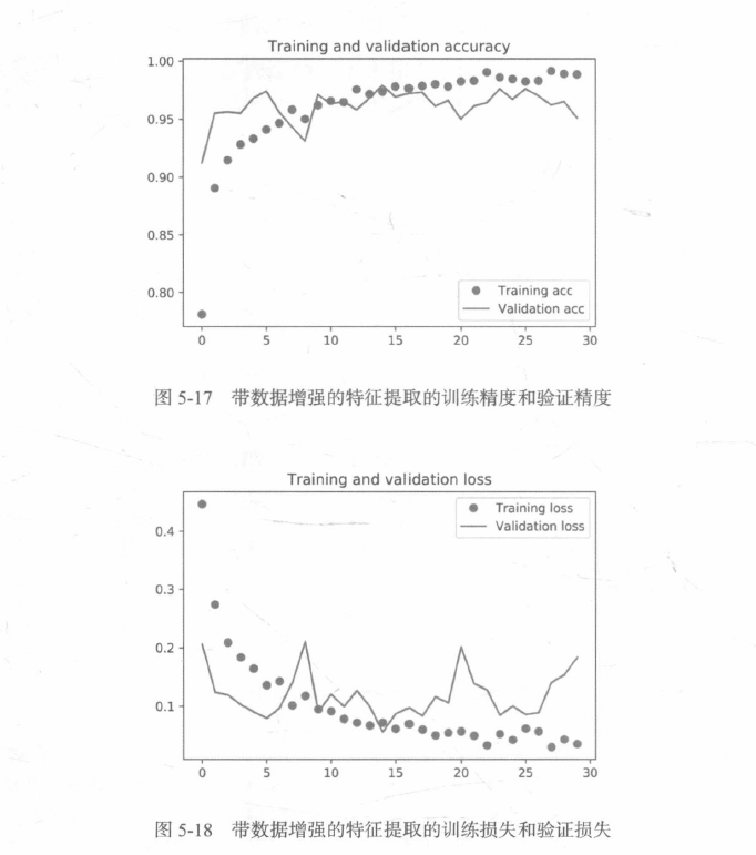
利用数据增强生成器训练卷积神经网络:
# 利用数据增强生成训练卷积神经网络
train_datagen = ImageDataGenerator(
    rescale=1./255,
    rotation_range=40,
    width_shift_range=0.2,
    height_shift_range=0.2,
    shear_range=0.2,
    zoom_range=0.2,
    horizontal_flip=True,
)

test_datagen = ImageDataGenerator(rescale=1./255)  # 注意,不能增强验证数据

train_generator = train_datagen.flow_from_directory(
    train_dir,  # 目标目录
    target_size=(150, 150),  # 将所有图像的大小调整为150x150
    batch_size=32,
    class_mode='binary'  # 因为使用了binary_crossentropy损失,所以需要用二进制标签
)

validation_generator = test_datagen.flow_from_directory(
    validation_dir,
    target_size=(150, 150),
    batch_size=32,
    class_mode='binary'
)

history = model.fit(
    train_generator,
    steps_per_epoch=100,
    epochs=100,
    validation_data=validation_generator,
    validation_steps=50
)
保存模型:
# 保存模型
model.save('cats_and_dogs_small_2.h5')
我们再次绘制结果:
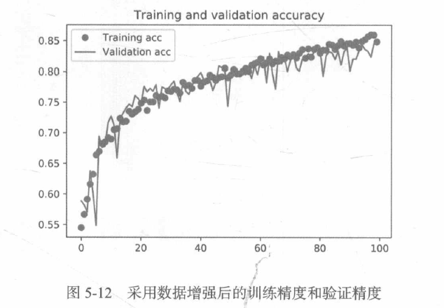
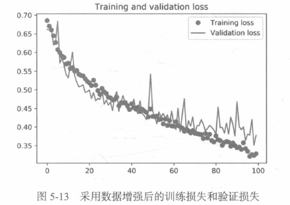
通过进一步使用正则化方法以及调节网络参数(比如每个卷积层的过滤器个数或网络中的层数),你可以得到更高的精度,但只靠从头开始训练自己的卷积神经网络,再想提高精度就十分困难,因为可用的数据太少。想要在这个问题上进一步提高精度,下一步需要使用预训练的模型。
5.3 使用预训练的卷积神经网络
想要将深度学习应用于小型图像数据集,一种常用且非常高效的方法是使用预训练网络。预训练网络是一个保存好的网络,之前已在大型数据集(通常是大规模图像分类任务) 上训练好。如果这个原始数据集足够大且足够通用,那么预训练网络学到的特征的空间层次结构可以有效地作为视觉世界的通用模型,因此这些特征可用于各种不同的计算机视觉问题,即使这些新问题涉及的类别和原始任务完全不同。
使用预训练网络有两种方法:特征提取和微调模型。
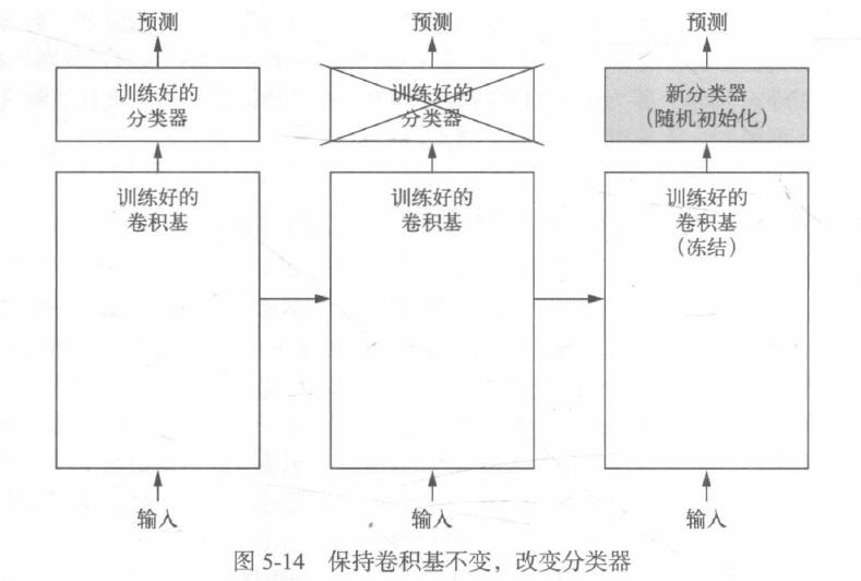
5.3.1 特征提取
特征提取是使用之前网络学到的表示来从新样本中提取出有趣的特征,然后将这些特征输入一个新的分类器,从头开始训练。
用于图像分类的卷积神经网络包含两部分:首先是一系列池化层和卷积层,最后是一个密集连接分类器。第一部分叫作模型的卷积基。对于卷积神经网络而言,特征提取就是取出之前训练好的网络的卷积基,在上面运行新数据,然后在输出上面训练的一个新的分类器。
卷积基学到的表示可能更加通用,因此更适合重复使用。卷积神经网络的特征图表示通用概念在图像中是否存在,无论面对什么样的计算机视觉问题,这种特征图都可能很有用。但是,分类器学到的表示必然是针对于模型训练的类别,其中仅包含某个类别出现在整张图像中的概率信息。此外,密集连接层的表示不再包含物体在输入图像中的位置信息。密集连接层舍弃了空间的概念,而物体位置信息仍然由卷积特征图所描述。如果物体位置对于问题很重要,那么密集连接层的特征在很大程度上是无用的。
某个卷积层提取的表示的通用性(以及可复用性)取决于该层在模型中的深度。模型中更靠近底部的层提取的是局部的、高度通用的特征图(比如视觉边缘、颜色和纹理),而更靠近顶部的层提取的是更加抽象的概念(比如“猫耳朵”或“狗眼睛”) 。因此,如果你的新数据集与原始模型训练的数据集有很大差异,那么最好只使用模型的前几层来做特征提取,而不是使用整个卷积基。
将VGG16卷积基实例化:
from keras.applications.vgg16 import VGG16

conv_base = VGG16(weights='imagenet',
                  include_top=False,
                  input_shape=(150, 150, 3))
print(conv_base.summary())
Model: "vgg16"
_________________________________________________________________
 Layer (type)                Output Shape              Param #
=================================================================
 input_1 (InputLayer)        [(None, 150, 150, 3)]     0

 block1_conv1 (Conv2D)       (None, 150, 150, 64)      1792

 block1_conv2 (Conv2D)       (None, 150, 150, 64)      36928

 block1_pool (MaxPooling2D)  (None, 75, 75, 64)        0

 block2_conv1 (Conv2D)       (None, 75, 75, 128)       73856

 block2_conv2 (Conv2D)       (None, 75, 75, 128)       147584

 block2_pool (MaxPooling2D)  (None, 37, 37, 128)       0

 block3_conv1 (Conv2D)       (None, 37, 37, 256)       295168

 block3_conv2 (Conv2D)       (None, 37, 37, 256)       590080

 block3_conv3 (Conv2D)       (None, 37, 37, 256)       590080

 block3_pool (MaxPooling2D)  (None, 18, 18, 256)       0

 block4_conv1 (Conv2D)       (None, 18, 18, 512)       1180160

 block4_conv2 (Conv2D)       (None, 18, 18, 512)       2359808

 block4_conv3 (Conv2D)       (None, 18, 18, 512)       2359808

 block4_pool (MaxPooling2D)  (None, 9, 9, 512)         0

 block5_conv1 (Conv2D)       (None, 9, 9, 512)         2359808

 block5_conv2 (Conv2D)       (None, 9, 9, 512)         2359808

 block5_conv3 (Conv2D)       (None, 9, 9, 512)         2359808

 block5_pool (MaxPooling2D)  (None, 4, 4, 512)         0

=================================================================
Total params: 14,714,688
Trainable params: 14,714,688
Non-trainable params: 0
_________________________________________________________________
None
最后的特征图形状为(4, 4, 512)。我们将在这个特征上添加一个密集连接分类器。下一步有两种方法可供选择:
(1)在你的数据集上运行卷积基,将输出保存成硬盘中的Numpy数组,然后用这个数据作为输入,输入到独立的密集连接分类其中。
(2)在顶部添加Dense层来扩展已有模型,并在输入数据上端到端地运行整个模型。
1.不使用数据增强的快速特征提取
# 使用预训练的卷积基提取特征
import os
import numpy as np
from keras.preprocessing.image import ImageDataGenerator
from keras.applications.vgg16 import VGG16

# 将VGG16卷积实例化
conv_base = VGG16(weights='imagenet',
                  include_top=False,
                  input_shape=(150, 150, 3))

base_dir = r'E:\train'
train_dir = os.path.join(base_dir, 'train')
validation_dir = os.path.join(base_dir, 'validation')
test_dir = os.path.join(base_dir, 'test')

datagen = ImageDataGenerator(rescale=1./255)
batch_size = 20

def extract_features(directory, sample_count):
    features = np.zeros(shape=(sample_count, 4, 4, 512))
    labels = np.zeros(shape=sample_count)
    generator = datagen.flow_from_diretory(
        directory,
        target_size=(150, 150),
        batch_size=batch_size,
        class_mode='binary'
    )
    i = 0
    for inputs_batch, labels_batch in generator:
        features_batch = conv_base.predict(inputs_batch)
        features[i * batch_size : (i + 1) * batch_size] = features_batch
        labels[i * batch_size : (i + 1) * batch_size] = labels_batch
        i += 1
        if i * batch_size >= sample_count:
            break
        if i * batch_size >= sample_count:
            break
    return features, labels

train_features, train_labels = extract_features(train_dir, 2000)
validation_features, validation_labels = extract_features(validation_dir, 1000)
test_features, test_labels = extract_features(test_dir, 1000)

# 将提取的特征形状展平为(samples, 8192)
train_features = np.reshape(train_features, (2000, 4 * 4 * 512))
validation_features = np.reshape(validation_features, (1000, 4 * 4 * 512))
test_features = np.reshape(test_features, (1000, 4 * 4 * 512))
定义并训练密集连接分类器:
from keras import models
from keras import layers
from tensorflow import optimizers

model = models.Sequential()
model.add(layers.Dense(256, activation='relu', input_dim=4 * 4 * 512))
model.add(layers.Dropout(0.5))
model.add(layers.Dense(1, activation='sigmoid'))

model.compile(optimizer=optimizers.RMSprop(lr=2e-5),
              loss='binary_crossentropy',
              metircs=['acc'])

history = model.fit(train_features, train_labels,
                    epochs=30,
                    batch_size=20,
                    validation_data=(validation_features, validation_labels))
绘制结果:
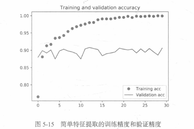
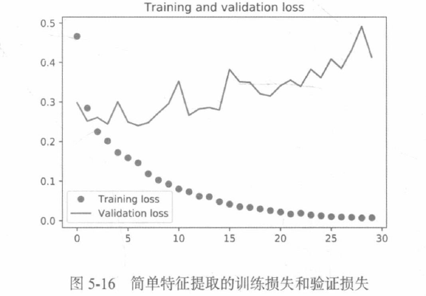
我们的验证精度达到了约90%,比从头开始训练的小型模型效果要好得多。从图中也可以看出,虽然dropout比率相当大,但模型几乎从一开始就过拟合。这是因为本方法没有使用数据增强,而数据增强对防止小型图像数据集的过拟合非常重要。
**2.使用数据增强的特征提取 **
扩展conv_base模型,然后在输入数据上端到端地运行模型。模型的行为和层类似,所以你可以向Sequential模型中添加一个模型(比如conv_base),就像添加一个层一样。
在卷积基上添加一个密集连接分类器:
from keras import models
from keras import layers
from keras.applications.vgg16 import VGG16

conv_base = VGG16(weights='imagenet',
                  include_top=False,
                  input_shape=(150, 150, 3))

model = models.Sequential()
model.add(conv_base)
model.add(layers.Flatten())
model.add(layers.Dense(256, activation='relu'))
model.add(layers.Dense(1, activation='sigmoid'))

print(model.summary())
Model: "sequential"
_________________________________________________________________
 Layer (type)                Output Shape              Param #
=================================================================
 vgg16 (Functional)          (None, 4, 4, 512)         14714688

 flatten (Flatten)           (None, 8192)              0

 dense (Dense)               (None, 256)               2097408

 dense_1 (Dense)             (None, 1)                 257

=================================================================
Total params: 16,812,353
Trainable params: 16,812,353
Non-trainable params: 0
_________________________________________________________________
None
在编译和训练模型之前,一定要“冻结”卷积基。冻结一个或多个层是指在训练过程中保持其权重不变。如果不这么做,那么卷积基之前学到的表示将会在训练过程中被修改。因为其上添加的Dense层是随机初始化的,所以非常大的权重更新将会在网络中传播,对之前学到的表示造成很大破坏。
print('This is the number of trainable weights before freezing the conv base:', len(model.trainable_weights))
conv_base.trainable = False
print('This is the number of trainable weights after freezing the conv base:', len(model.trainable_weights))
This is the number of trainable weights before freezing the conv base: 30
This is the number of trainable weights after freezing the conv base: 4
利用冻结的卷积基端到端地训练模型:
train_generator = train_datagen.flow_from_directory(
    train_dir,
    target_size=(150, 150),
    batch_size=20,
    class_mode='binary'
)

validation_generator = test_datagen.flow_from_directory(
    validation_dir,
    target_size=(150, 150),
    batch_size=20,
    class_mode='binary'
)

model.compile(loss='binary_crossentropy',
              optimizer=optimizers.RMSprop(lr=2e-5),
              metrics=['acc'])

history = model.fit_generator(
    train_generator,
    steps_per_epoch=100,
    epochs=30,
    validation_data=validation_generator,
    validation_steps=50
)
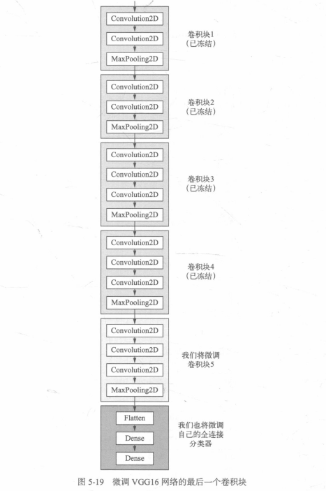
5.3.2 微调模型
另一种广泛使用的模型复用方法是模型微调,与特征提取互为补充。对于用于特征提取的冻结的模型基,微调是指将其顶部的几层“解冻”,并将这解冻的几层和新增加的部分联合训练。之所以叫作微调,是因为它只是略微调整了所复用模型中更加抽象的表示,以便让这些表示与手头的问题更加相关。
微调网络的步骤如下:
(1)在已经训练好的基网络上添加自定义网络;
(2)冻结基网络;
(3)训练所添加的部分;
(4)解冻基网络的一些层;
(5)联合训练解冻的这些层和添加的部分。
卷积基中更靠底部的层编码的是更加通用的可复用特征,而更靠顶部的层编码的是更专业化的特征。微调这些更专业化的特征更加有用,因为它们需要在你的新问题上改变用途。微调更靠底部的层,得到的回报会更少。
训练的参数越多,过拟合的风险越大。卷积基有1500万个参数,所以在你的小型数据集上训练这么多参数是有风险的。
冻结直到某一层的所有层:
# 冻结直到某一层的所有层
conv_base.trainable = True

set_trainable = False
for layer in conv_base.layers:
    if layer.name == 'block5_conv1':
        set_trainable = True
    if set_trainable:
        layer.trainable = True
    else:
        layer.trainable = False

# 微调模型
model.compile(loss='binary_crossentropy',
              optimizer=optimizers.RMSprop(lr=1e-5),
              metrics=['acc'])
history = model.fit_generator(
    train_generator,
    steps_per_epoch=100,
    epochs=100,
    validation_data=validation_generator,
    validation_steps=50
)
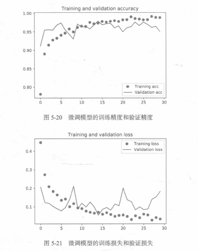
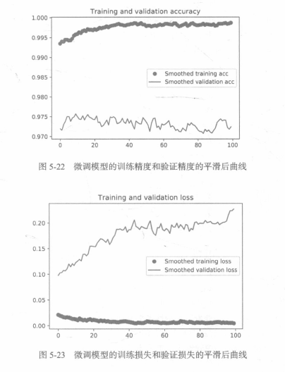
使曲线变得平滑:
# 使曲线变得平滑
def smooth_curve(points, factor=0.8):
    smoothed_points = []
    for point in points:
        if smoothed_points:
            previous = smoothed_points[-1]
            smoothed_points.append(previous * factor + point * (1 - factor))
        else:
            smoothed_points.append(point)
    return smoothed_points
test_generator = test_datagen.flow_from_directory(
    test_dir,
    target_size=(150, 150),
    batch_size=20,
    class_mode='binary'
)

test_loss, test_acc = model.evaluate_generator(test_generator, steps=50)
print('test acc:', test_acc)
5.3.3 小结
1.卷积神经网络是用于计算机视觉任务的最佳机器学习模型。即使在非常小的数据集上也可以从头开始训练一个卷积神经网络,而且得到的结果还不错。
2.在小型数据集上的主要问题是过拟合。在处理图像数据时,数据增强是一种降低过拟合的强大方法;
3.利用特征提取,可以很容易将现有的卷积神经网络复用于新的数据集,对于小型图像数据集,这是一种很有价值的方法;
4.作为特征提取的补充,你还可以使用微调,将现有模型之前学到的一些数据表示应用于新问题,这种方法可以进一步提高模型性能。
5.4 卷积神经网络的可视化
人们常说,深度学习模型是“黑盒”, 即模型学到的表示很难用人类可以理解的方式来提取和呈现。虽然对于某些类型的深度学习模型来说,这种说法部分正确,但对卷积神经网络来说绝不是这样。卷积神经网络学到的表示非常适合可视化,很大程度上是因为它们是视觉概念的表示。
三种最容易理解也最有用的对这些表示进行可视化和解释的方法:
1.可视化卷积神经网络的中间输出(中间激活);
2.可视化卷积神经网络的过滤器;
3.可视化图像中类激活的热力图。
5.4.1 可视化中间激活
可视化中间激活,是指对于给定输入,展示网络中各个卷积层和池化层输出的特征图(层的输出通常被称为该层的激活,即激活函数的输出)。这让我们可以看到输入如何被分解为网络学到的不同过滤器。
(这一章的代码实现遇到了一些问题,暂且跳过这一章,先进入下一章的学习)
有木有大佬能够帮忙解答一下如下问题:
使用如下代码导入optimizers
from keras import optimizers
运行后显示:
AttributeError: module 'keras.optimizers' has no attribute 'RMSprop'
将导入方式改成如下:
from tensorflow import optimizers
则又显示:
AttributeError: module 'tensorflow.compat.v2.__internal__.distribute' has no attribute 'strategy_supports_no_merge_call'
请问如何解决?
版权归原作者 feiwen110 所有, 如有侵权,请联系我们删除。