
图像分类🍉
文章目录
前言🎠
上一章介绍了深度学习的基础内容,这一章来学习一下图像分类的内容。图像分类是计算机视觉中最基础的一个任务,也是几乎所有的基准模型进行比较的任务。从最开始比较简单的10分类的灰度图像手写数字识别任务mnist,到后来更大一点的10分类的 cifar10和100分类的cifar100 任务,到后来的imagenet 任务,图像分类模型伴随着数据集的增长,一步一步提升到了今天的水平。现在,在imagenet 这样的超过1000万图像,超过2万类的数据集中,计算机的图像分类水准已经超过了人类。
一、ILSVRC竞赛
ILSVRC(ImageNet Large Scale Visual Recognition Challenge)是近年来机器视觉领域最受追捧也是最具权威的学术竞赛之一,代表了图像领域的最高水平。ILSVRC竞赛使得深度学习算法得到大力的发展,AI领域迎来了新一轮的热潮,CNN网络也不断迭代,图像分类的准确度也逐年上升,最终超越人类,完成竞赛的使命,2017年已经停办。
ImageNet数据集是ILSVRC竞赛使用的是数据集,由斯坦福大学李飞飞教授主导,包含了超过1400万张全尺寸的有标记图片。ILSVRC比赛会每年从ImageNet数据集中抽出部分样本,以2012年为例,比赛的训练集包含1281167张图片,验证集包含50000张图片,测试集为100000张图片。
卷积神经网络在特征表示上具有极大的优越性,模型提取的特征随着网络深度的增加越来越抽象,越来越能表现图像主题语义,不确定性越少,识别能力越强。AlexNet 的成功证明了CNN 网络能够提升图像分类的效果,其使用了 8 层的网络结构,获得了 2012 年,ImageNet 数据集上图像分类的冠军,为训练深度卷积神经网络模型提供了参考。2014 年,冠军 GoogleNet 另辟蹊径,从设计网络结构的角度来提升识别效果。其主要贡献是设计了 Inception 模块结构来捕捉不同尺度的特征,通过 1×1 的卷积来进行降维。2014 年另外一个工作是 VGG(亚军),进一步证明了网络的深度在提升模型效果方面的重要性。2015 年,最重要的一篇文章是关于深度残差网络 ResNet ,文章提出了拟合残差网络的方法,能够做到更好地训练更深层的网络。 2017年,SENet是ImageNet(ImageNet收官赛)的冠军模型,和ResNet的出现类似,都在很大程度上减小了之前模型的错误率),并且复杂度低,新增参数和计算量小。
历届冠军做法: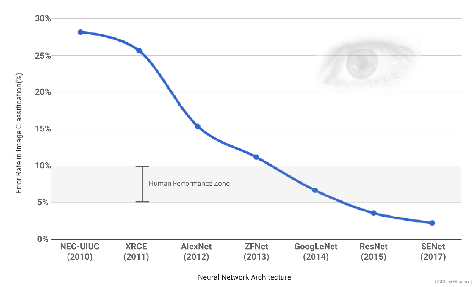
二、卷积神经网络(CNN)发展
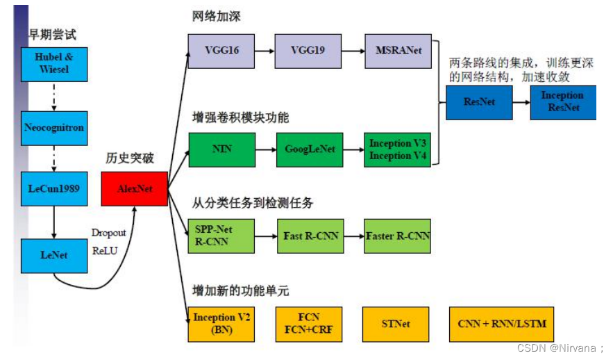
1.网络进化
🎄网络:AlexNet–>VGG–>GoogLeNet–>ResNet
🎨深度:8–>19–>22–>152
✨VGG结构简洁有效
- 容易修改,迁移到其他任务中
- 高层任务的基础网络
🖼️性能竞争网络
- GoogLeNet:Inception v1–>v4 - Split-transform-merge
- ResNet:ResNet1024–>ResNeXt - 深度、宽度、基数
2.AlexNet网络
由于受到计算机性能的影响,虽然LeNet在图像分类中取得了较好的成绩,但是并没有引起很多的关注。 知道2012年,Alex等人提出的AlexNet网络在ImageNet大赛上以远超第二名的成绩夺冠,卷积神经网络乃至深度学习重新引起了广泛的关注。
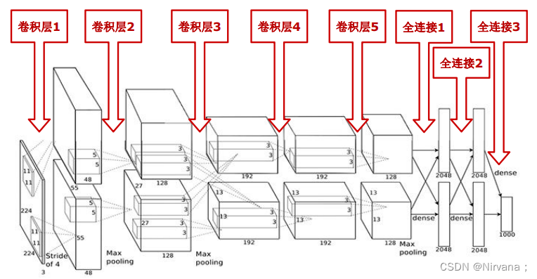
- AlexNet包含8层网络,有5个卷积层和3个全连接层
- AlexNet第一层中的卷积核shape为11X11,第二层的卷积核形状缩小到5X5,之后全部采用3X3的卷积核
- 所有的池化层窗口大小为3X3,步长为2,最大池化采用Relu激活函数,代替sigmoid,梯度计算更简单,模型更容易训练
- 采用Dropout来控制模型复杂度,防止过拟合采用大量图像增强技术,比如翻转、裁剪和颜色变化,扩大数据集,防止过拟合
 代码实现
代码实现
# 导入工具包import tensorflow as tf
from tensorflow import keras
from tensorflow.keras import layers

# 模型构建
net = keras.models.Sequential([# 卷积:卷积核数量96,尺寸11*11,步长4,激活函数relu
    layers.Conv2D(filters=96, kernel_size=11, strides=4, activation='relu'),# 最大池化:尺寸3*3,步长2
    layers.MaxPool2D(pool_size=3, strides=2),# 卷积:卷积核数量256,尺寸5*5,激活函数relu,same卷积
    layers.Conv2D(filters=256, kernel_size=5, padding='same', activation='relu'),# 最大池化:尺寸3*3,步长3
    layers.MaxPool2D(pool_size=3, strides=2),# 卷积:卷积核数量384,尺寸3,激活函数relu,same卷积
    layers.Conv2D(filters=384, kernel_size=3, padding='same', activation='relu'),# 卷积:卷积核数量384,尺寸3,激活函数relu,same卷积
    layers.Conv2D(filters=384, kernel_size=3, padding='same', activation='relu'),# 卷积:卷积核数量256,尺寸3,激活函数relu,same卷积
    layers.Conv2D(filters=256, kernel_size=3, padding='same', activation='relu'),# 最大池化:尺寸3*3,步长2
    layers.MaxPool2D(pool_size=3, strides=2),# 展平特征图
    layers.Flatten(),# 全连接:4096神经元,relu
    layers.Dense(4096, activation='relu'),# 随机失活
    layers.Dropout(0.5),
    layers.Dense(4096, activation='relu'),
    layers.Dropout(0.5),# 输出层:多分类用softmax,二分类用sigmoid
    layers.Dense(10, activation='softmax')],
    name='AlexNet')# 模拟输入
x = tf.random.uniform((1,227,227,1))
y = net(x)

net.summary()
3.VGG网络
VGG网络是在2014年由牛津大学计算机视觉组和谷歌公司的研究员共同开发的。VGG由5层卷积层、3层全连接层、softmax输出层构成,层与层之间使用最大池化分开,所有隐层的激活单元都采用ReLU函数。通过反复堆叠3X3的小卷积核和2X2的最大池化层,VGGNet成功的搭建了16-19层的深度卷积神经网络。VGG的结构图如下: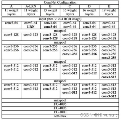
VGGNet 论文中全部使用了3X3的卷积核和2X2的池化核,通过不断加深网络结构来提升性能。下图所示为 VGGNet 各级别的网络结构图,以及随后的每一级别的参数量,从11层的网络一直到19层的网络都有详尽的性能测试。虽然从A到E每一级网络逐渐变深,但是网络的参数量并没有增长很多,这是因为参数量主要都消耗在最后3个全连接层。前面的卷积部分虽然很深,但是消耗的参数量不大,不过训练比较耗时的部分依然是卷积,因其计算量比较大。这其中的D、E也就是我们常说的 VGGNet-16 和 VGGNet-19。C相比B多了几个1X1的卷积层,1X1卷积的意义主要在于线性变换,而输入通道数和输出通道数不变,没有发生降维。
代码实现 VGG11
#tensorflow基于mnist数据集上的VGG11网络,可以直接运行from tensorflow.examples.tutorials.mnist import input_data
import tensorflow as tf
#tensorflow基于mnist实现VGG11
mnist = input_data.read_data_sets('MNIST_data', one_hot=True)

x = tf.placeholder(tf.float32,[None,784])
y_ = tf.placeholder(tf.float32,[None,10])
sess = tf.InteractiveSession()#Layer1
W_conv1 =tf.Variable(tf.truncated_normal([3,3,1,64],stddev=0.1))
b_conv1 = tf.Variable(tf.constant(0.1,shape=[64]))#调整x的大小
x_image = tf.reshape(x,[-1,28,28,1])
h_conv1 = tf.nn.relu(tf.nn.conv2d(x_image, W_conv1,strides=[1,1,1,1], padding='SAME')+ b_conv1)#Layer2 pooling
W_conv2 = tf.Variable(tf.truncated_normal([3,3,64,64],stddev=0.1))
b_conv2 = tf.Variable(tf.constant(0.1,shape=[64]))
h_conv2 = tf.nn.relu(tf.nn.conv2d(h_conv1, W_conv2,strides=[1,1,1,1], padding='SAME')+ b_conv2)
h_pool2 = tf.nn.max_pool(h_conv2, ksize=[1,2,2,1],
                        strides=[1,2,2,1], padding='SAME')#Layer3
W_conv3 = tf.Variable(tf.truncated_normal([3,3,64,128],stddev=0.1))
b_conv3 = tf.Variable(tf.constant(0.1,shape=[128]))
h_conv3 = tf.nn.relu(tf.nn.conv2d(h_pool2, W_conv3,strides=[1,1,1,1], padding='SAME')+ b_conv3)#Layer4 pooling
W_conv4 = tf.Variable(tf.truncated_normal([3,3,128,128],stddev=0.1))
b_conv4 = tf.Variable(tf.constant(0.1,shape=[128]))
h_conv4 = tf.nn.relu(tf.nn.conv2d(h_conv3, W_conv4,strides=[1,1,1,1], padding='SAME')+ b_conv4)
h_pool4= tf.nn.max_pool(h_conv4, ksize=[1,2,2,1],
                        strides=[1,2,2,1], padding='SAME')#Layer5
W_conv5 = tf.Variable(tf.truncated_normal([3,3,128,256],stddev=0.1))
b_conv5 = tf.Variable(tf.constant(0.1,shape=[256]))
h_conv5 = tf.nn.relu(tf.nn.conv2d(h_pool4, W_conv5,strides=[1,1,1,1], padding='SAME')+ b_conv5)#Layer6
W_conv6 = tf.Variable(tf.truncated_normal([3,3,256,256],stddev=0.1))
b_conv6 = tf.Variable(tf.constant(0.1,shape=[256]))
h_conv6 = tf.nn.relu(tf.nn.conv2d(h_conv5, W_conv6,strides=[1,1,1,1], padding='SAME')+ b_conv6)#Layer7
W_conv7 = tf.Variable(tf.truncated_normal([3,3,256,256],stddev=0.1))
b_conv7 = tf.Variable(tf.constant(0.1,shape=[256]))
h_conv7 = tf.nn.relu(tf.nn.conv2d(h_conv6, W_conv7,strides=[1,1,1,1], padding='SAME')+ b_conv7)#Layer8
W_conv8 = tf.Variable(tf.truncated_normal([3,3,256,256],stddev=0.1))
b_conv8 = tf.Variable(tf.constant(0.1,shape=[256]))
h_conv8 = tf.nn.relu(tf.nn.conv2d(h_conv7, W_conv8,strides=[1,1,1,1], padding='SAME')+ b_conv8)
h_pool8 = tf.nn.max_pool(h_conv8, ksize=[1,2,2,1],
                        strides=[1,1,1,1], padding='SAME')#Layer9-全连接层
W_fc1 = tf.Variable(tf.truncated_normal([7*7*256,1024],stddev=0.1))
b_fc1 = tf.Variable(tf.constant(0.1,shape=[1024]))#对h_pool2数据进行铺平
h_pool2_flat = tf.reshape(h_pool8,[-1,7*7*256])#进行relu计算,matmul表示(wx+b)计算
h_fc1 = tf.nn.relu(tf.matmul(h_pool2_flat, W_fc1)+ b_fc1)
keep_prob = tf.placeholder(tf.float32)
h_fc1_drop = tf.nn.dropout(h_fc1, keep_prob)#Layer10-全连接层,这里也可以是[1024,其它],大家可以尝试下
W_fc2 = tf.Variable(tf.truncated_normal([1024,1024],stddev=0.1))
b_fc2 = tf.Variable(tf.constant(0.1,shape=[1024]))
h_fc2 = tf.nn.relu(tf.matmul(h_fc1_drop, W_fc2)+ b_fc2)
h_fc2_drop = tf.nn.dropout(h_fc2, keep_prob)#Layer11-softmax层
W_fc3 = tf.Variable(tf.truncated_normal([1024,10],stddev=0.1))
b_fc3 = tf.Variable(tf.constant(0.1,shape=[10]))
y_conv = tf.matmul(h_fc2_drop, W_fc3)+ b_fc3
#在这里通过tf.nn.softmax_cross_entropy_with_logits函数可以对y_conv完成softmax计算,同时计算交叉熵损失函数
cross_entropy = tf.reduce_mean(
    tf.nn.softmax_cross_entropy_with_logits(labels=y_, logits=y_conv))#定义训练目标以及加速优化器
train_step = tf.train.AdamOptimizer(1e-3).minimize(cross_entropy)#计算准确率
correct_prediction = tf.equal(tf.argmax(y_conv,1), tf.argmax(y_,1))
accuracy = tf.reduce_mean(tf.cast(correct_prediction, tf.float32))#初始化变量
saver = tf.train.Saver()
sess.run(tf.global_variables_initializer())for i inrange(20000):
  batch = mnist.train.next_batch(10)if i%100==0:
    train_accuracy = accuracy.eval(feed_dict={
        x:batch[0], y_: batch[1], keep_prob:1.0})print("step %d, training accuracy %g"%(i, train_accuracy))
  train_step.run(feed_dict={x: batch[0], y_: batch[1], keep_prob:0.5})#保存模型
save_path = saver.save(sess,"./model/save_net.ckpt")print("test accuracy %g"%accuracy.eval(feed_dict={
    x: mnist.test.images[:3000], y_: mnist.test.labels[:3000], keep_prob:1.0}))
4.GoogLeNet网络
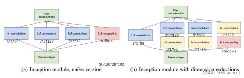
Google Inception Net通常被称为Google Inception V1,在ILSVRC-2014比赛中由论文<Going deeper with convolutions>提出.
Inception V1有22层,比AlexNet的8层和VGGNet的19层还要深.参数量(500万)仅有AlexNet参数量(6000万)的1/12,但准确率远胜于AlexNet的准确率.
Inception V1降低参数量的目的:
- 参数越多模型越庞大,需要模型学习的数据量就越大,且高质量的数据非常昂贵.
- 参数越多,消耗的计算资源越多.
Inception V1网络的特点:
- 模型层数更深(22层),表达能力更强.
- 去除最后的全连接层,用全局平均池化层(即将图片尺寸变为1X1)来代替它.(借鉴了NIN)
- 使用Inception Module提高了参数利用效率.
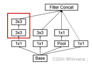
 Inception V2网络的特点:
 - Batch Normalization 白化:使每一层的输出都规范化到N(0,1)
- 解决Interal Covariate Shift问题
- 允许较高学习率
- 取代部分Dropout
- 5X5卷积核–>2个3X3卷积核
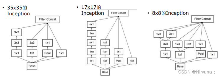
Inception V3网络的特点:
- 高效的降尺寸
- 不增加计算量
- 取消浅层的辅助分类器
- 深层辅助分类器只在训练后期有用
GoogLeNet网络结构: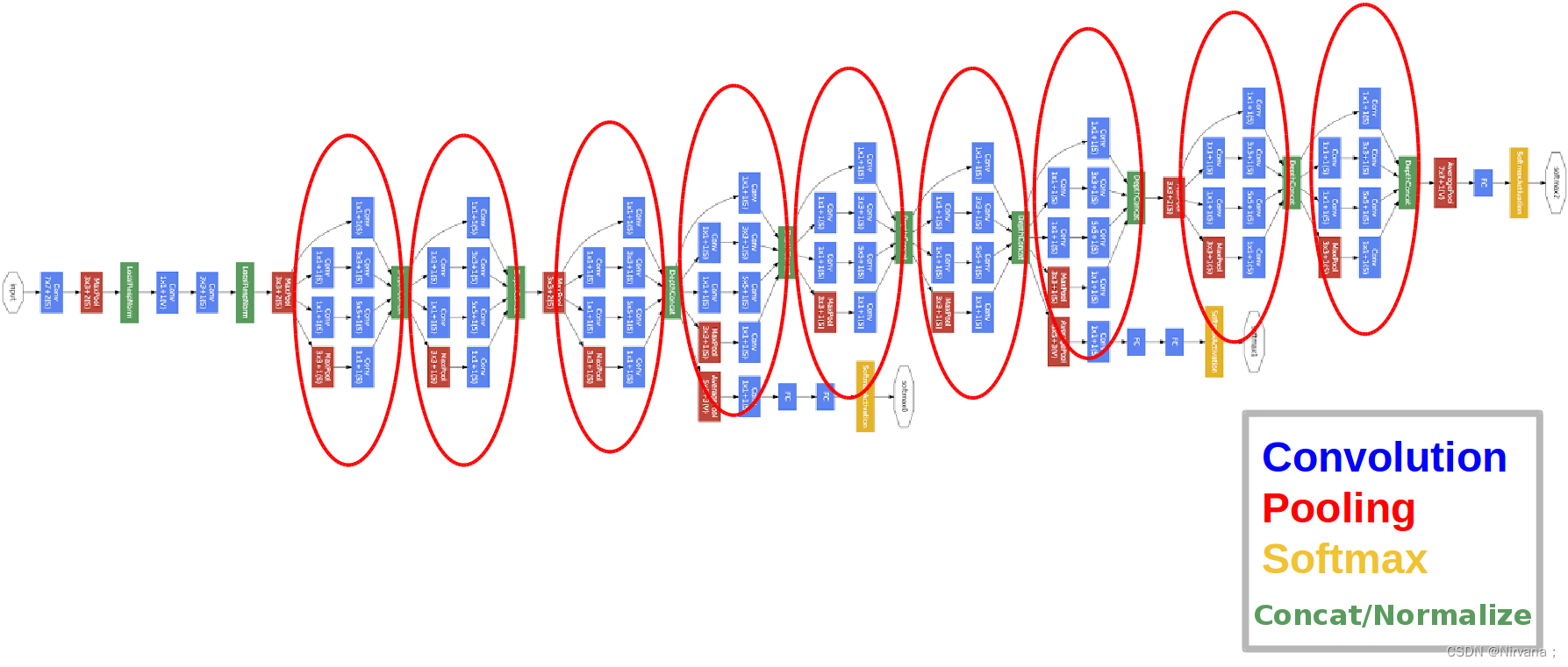
对于我们搭建的Inception模块,所需要使用到参数有#1x1, #3x3reduce, #3x3, #5x5reduce, #5x5, poolproj,这6个参数,分别对应着所使用的卷积核个数,参数设置如下表所示: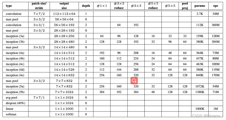
代码实现 Inception V3
import tensorflow as tf
slim = tf.contrib.slim
trunc_normal =lambda stddev: tf.truncated_normal_initializer(0.0, stddev)# 生成默认参数definception_v3_arg_scope(weight_decay=0.00004,# L2正则weight_decay
                           stddev=0.1,# 标准差
                           batch_norm_var_collection='moving_vars'):
    batch_norm_params ={'decay':0.9997,'epsilon':0.001,'updates_collections': tf.GraphKeys.UPDATE_OPS,'variables_collections':{'beta':None,'gamma':None,'moving_mean':[batch_norm_var_collection],'moving_variance':[batch_norm_var_collection],}}# 提供了新的范围名称scope name# 对slim.conv2d和slim.fully_connected两个函数的参数自动赋值with slim.arg_scope([slim.conv2d, slim.fully_connected],
                        weights_regularizer=slim.l2_regularizer(weight_decay)):with slim.arg_scope([slim.conv2d],# 对卷积层的参数赋默认值
            weights_initializer=tf.truncated_normal_initializer(stddev=stddev),# 权重初始化器
            activation_fn=tf.nn.relu,# 激活函数用ReLU
            normalizer_params=batch_norm_params)as sc:# 标准化器参数用batch_norm_paramsreturn sc

# inputs为输入图片数据的tensor(299x299x3),scope为包含了函数默认参数的环境definception_v3_base(inputs, scope=None):# 保存某些关键节点
    end_points ={}# 定义InceptionV3的网络结构with tf.variable_scope(scope,'InceptionV3',[inputs]):# 设置卷积/最大池化/平均池化的默认步长为1,padding模式为VALID# 设置Inception模块组的默认参数with slim.arg_scope([slim.conv2d,# 创建卷积层
                             slim.max_pool2d,# 输出的通道数
                             slim.avg_pool2d],# 卷积核尺寸
                            stride=1,# 步长
                            padding='VALID'):# padding模式# 经3个3x3的卷积层后,输入数据(299x299x3)变为(35x35x192),空间尺寸降低,输出通道增加
            net = slim.conv2d(inputs,32,[3,3], stride=2, scope='Conv2d_1a_3x3')
            net = slim.conv2d(net,32,[3,3], scope='Conv2d_2a_3x3')
            net = slim.conv2d(net,64,[3,3], padding='SAME', scope='Conv2d_2b_3x3')

            net = slim.max_pool2d(net,[3,3], stride=2, scope='MaxPool_3a_3x3')
            net = slim.conv2d(net,80,[1,1], scope='Conv2d_3b_1x1')
            net = slim.conv2d(net,192,[3,3], scope='Conv2d_4a_3x3')
            net = slim.max_pool2d(net,[3,3], stride=2, scope='MaxPool_5a_3x3')# 设置卷积/最大池化/平均池化的默认步长为1,padding模式为SAME# 步长为1,padding模式为SAME,所以图像尺寸不会变,仍为35x35with slim.arg_scope([slim.conv2d, slim.max_pool2d, slim.avg_pool2d], stride=1, padding='SAME'):# 设置Inception Moduel名称为Mixed_5bwith tf.variable_scope('Mixed_5b'):# 第1个分支:64输出通道的1x1卷积with tf.variable_scope('Branch_0'):
                    branch_0 = slim.conv2d(net,64,[1,1], scope='Conv2d_0a_1x1')# 第2个分支:48输出通道的1x1卷积,连接64输出通道的5x5卷积with tf.variable_scope('Branch_1'):
                    branch_1 = slim.conv2d(net,48,[1,1], scope='Con2d_0a_1x1')
                    branch_1 = slim.conv2d(branch_1,64,[5,5], scope='Conv2d_0b_5x5')# 第3个分支:64输出通道的1x1卷积,连接两个96输出通道的3x3卷积with tf.variable_scope('Branch_2'):
                    branch_2 = slim.conv2d(net,64,[1,1], scope='Conv2d_0a_1x1')
                    branch_2 = slim.conv2d(branch_2,96,[3,3], scope='Conv2d_0b_3x3')
                    branch_2 = slim.conv2d(branch_2,96,[3,3], scope='Conv2d_0c_3x3')# 第4个分支:3x3的平均池化,连接32输出通道的1x1卷积with tf.variable_scope('Branch_3'):
                    branch_3 = slim.avg_pool2d(net,[3,3], scope='AvgPool_0a_3x3')
                    branch_3 = slim.conv2d(branch_3,32,[1,1], scope='Conv2d_0b_1x1')# 4个分支输出通道数之和=64+64+96+32=256,输出tensor为35x35x256
                net = tf.concat([branch_0, branch_1, branch_2, branch_3],3)# 第1个Inception模块组的第2个Inception Modulewith tf.variable_scope('Mixed_5c'):# 第1个分支:64输出通道的1x1卷积with tf.variable_scope('Branch_0'):
                    branch_0 = slim.conv2d(net,64,[1,1], scope='Conv2d_0a_1x1')# 第2个分支:48输出通道的1x1卷积,连接64输出通道的5x5卷积with tf.variable_scope('Branch_1'):
                    branch_1 = slim.conv2d(net,48,[1,1], scope='Conv2d_0b_1x1')
                    branch_1 = slim.conv2d(branch_1,64,[5,5], scope='Conv2d_0c_5x5')# 第3个分支:64输出通道的1x1卷积,连接两个96输出通道的3x3卷积with tf.variable_scope('Branch_2'):
                    branch_2 = slim.conv2d(net,64,[1,1], scope='Conv2d_0a_1x1')
                    branch_2 = slim.conv2d(branch_2,96,[3,3], scope='Conv2d_0b_3x3')
                    branch_2 = slim.conv2d(branch_2,96,[3,3], scope='Conv2d_0c_3x3')# 第4个分支:3x3的平均池化,连接64输出通道的1x1卷积with tf.variable_scope('Branch_3'):
                    branch_3 = slim.avg_pool2d(net,[3,3], scope='AvgPool_0a_3x3')
                    branch_3 = slim.conv2d(branch_3,64,[1,1], scope='Conv2d_0b_1x1')# 输出tensor尺寸为35x35x288
                net = tf.concat([branch_0, branch_1, branch_2, branch_3],3)# 第1个Inception模块组的第3个Inception Modulewith tf.variable_scope('Mixed_5d'):# 第1个分支:64输出通道的1x1卷积with tf.variable_scope('Branch_0'):
                    branch_0 = slim.conv2d(net,64,[1,1], scope='Conv2d_0a_1x1')# 第2个分支:48输出通道的1x1卷积,连接64输出通道的5x5卷积with tf.variable_scope('Branch_1'):
                    branch_1 = slim.conv2d(net,48,[1,1], scope='Conv2d_0a_1x1')
                    branch_1 = slim.conv2d(branch_1,64,[5,5], scope='Conv2d_0b_5x5')# 第3个分支:64输出通道的1x1卷积,连接两个96输出通道的3x3卷积with tf.variable_scope('Branch_2'):
                    branch_2 = slim.conv2d(net,64,[1,1], scope='Conv2d_0a_1x1')
                    branch_2 = slim.conv2d(branch_2,96,[3,3], scope='Conv2d_0b_3x3')
                    branch_2 = slim.conv2d(branch_2,96,[3,3], scope='Conv2d_0c_3x3')# 第4个分支:3x3的平均池化,连接64输出通道的1x1卷积with tf.variable_scope('Branch_3'):
                    branch_3 = slim.avg_pool2d(net,[3,3], scope='AvgPool_0a_3x3')
                    branch_3 = slim.conv2d(branch_3,64,[1,1], scope='Conv2d_0b_1x1')# 输出tensor尺寸为35x35x288
                net = tf.concat([branch_0, branch_1, branch_2, branch_3],3)# 第2个Inception模块组with tf.variable_scope('Mixed_6a'):# 第1个分支:3x3卷积,步长为2,padding模式为VALID,因此图像被压缩为17x17with tf.variable_scope('Branch_0'):
                    branch_0 = slim.conv2d(net,384,[3,3], stride=2, padding='VALID', scope='Conv2d_1a_1x1')# 第2个分支:64输出通道的1x1卷积,连接2个96输出通道的3x3卷积with tf.variable_scope('Branch_1'):
                    branch_1 = slim.conv2d(net,64,[1,1], scope='Conv2d_0a_1x1')
                    branch_1 = slim.conv2d(branch_1,96,[3,3], scope='Conv2d_0b_3x3')# 步长为2,padding模式为VALID,因此图像被压缩为17x17
                    branch_1 = slim.conv2d(branch_1,96,[3,3], stride=2, padding='VALID', scope='Conv2d_1a_1x1')# 第3个分支:3x3的最大池化层,步长为2,padding模式为VALID,因此图像被压缩为17x17x256with tf.variable_scope('Branch_2'):
                    branch_2 = slim.max_pool2d(net,[3,3], stride=2, padding='VALID', scope='MaxPool_1a_3x3')
                net = tf.concat([branch_0, branch_1, branch_2],3)# 第2个Inception模块组,包含5个Inception Modulewith tf.variable_scope('Mixed_6b'):# 第1个分支:192输出通道的1x1卷积with tf.variable_scope('Branch_0'):
                    branch_0 = slim.conv2d(net,192,[1,1], scope='Conv2d_0a_1x1')# 第2个分支:128输出通道的1x1卷积,接128输出通道的1x7卷积,接192输出通道的7x1卷积with tf.variable_scope('Branch_1'):
                    branch_1 = slim.conv2d(net,128,[1,1], scope='Conv2d_0a_1x1')
                    branch_1 = slim.conv2d(branch_1,128,[1,7], scope='Conv2d_0b_1x7')
                    branch_1 = slim.conv2d(branch_1,192,[7,1], scope='Conv2d_0c_7x1')with tf.variable_scope('Branch_2'):
                    branch_2 = slim.conv2d(net,128,[1,1], scope='Conv2d_0a_1x1')
                    branch_2 = slim.conv2d(branch_2,128,[7,1], scope='Conv2d_0b_7x1')
                    branch_2 = slim.conv2d(branch_2,128,[1,7], scope='Conv2d_0c_1x7')
                    branch_2 = slim.conv2d(branch_2,128,[7,1], scope='Conv2d_0d_7x1')
                    branch_2 = slim.conv2d(branch_2,192,[1,7], scope='Conv2d_0e_1x7')with tf.variable_scope('Branch_3'):
                    branch_3 = slim.avg_pool2d(net,[3,3], scope='AvgPool_0a_3x3')
                    branch_3 = slim.conv2d(branch_3,192,[1,1], scope='Conv2d_0b_1x1')# 输出tensor尺寸=17x17x(192+192+192+192)=17x17x768
                net = tf.concat([branch_0, branch_1, branch_2, branch_3],3)# 经过一个Inception Module输出tensor尺寸不变,但特征相当于被精炼类一遍# 第3个Inception模块组with tf.variable_scope('Mixed_6c'):with tf.variable_scope('Branch_0'):
                    branch_0 = slim.conv2d(net,192,[1,1], scope='Conv2d_0a_1x1')with tf.variable_scope('Branch_1'):
                    branch_1 = slim.conv2d(net,160,[1,1], scope='Conv2d_0a_1x1')
                    branch_1 = slim.conv2d(branch_1,160,[1,7], scope='Conv2d_0b_1x7')
                    branch_1 = slim.conv2d(branch_1,192,[7,1], scope='Conv2d_0c_7x1')with tf.variable_scope('Branch_2'):
                    branch_2 = slim.conv2d(net,160,[1,1], scope='Conv2d_0a_1x1')
                    branch_2 = slim.conv2d(branch_2,160,[7,1], scope='Conv2d_0b_7x1')
                    branch_2 = slim.conv2d(branch_2,160,[1,7], scope='Conv2d_0c_1x7')
                    branch_2 = slim.conv2d(branch_2,160,[7,1], scope='Conv2d_0d_7x1')
                    branch_2 = slim.conv2d(branch_2,192,[1,7], scope='Conv2d_0e_1x7')with tf.variable_scope('Branch_3'):
                    branch_3 = slim.avg_pool2d(net,[3,3], scope='AvgPool_0a_3x3')
                    branch_3 = slim.conv2d(branch_3,192,[1,1], scope='Conv2d_0b_1x1')# 输出tensor尺寸为17x17x768
                net = tf.concat([branch_0, branch_1, branch_2, branch_3],3)# 第4个Inception模块组with tf.variable_scope('Mixed_6d'):with tf.variable_scope('Branch_0'):
                    branch_0 = slim.conv2d(net,192,[1,1], scope='Conv2d_0a_1x1')with tf.variable_scope('Branch_1'):
                    branch_1 = slim.conv2d(net,160,[1,1], scope='Conv2d_0a_1x1')
                    branch_1 = slim.conv2d(branch_1,160,[1,7], scope='Conv2d_0b_1x7')
                    branch_1 = slim.conv2d(branch_1,192,[7,1], scope='Conv2d_0c_7x1')with tf.variable_scope('Branch_2'):
                    branch_2 = slim.conv2d(net,160,[1,1], scope='Conv2d_0a_1x1')
                    branch_2 = slim.conv2d(branch_2,160,[7,1], scope='Conv2d_0b_7x1')
                    branch_2 = slim.conv2d(branch_2,160,[1,7], scope='Conv2d_0c_1x7')
                    branch_2 = slim.conv2d(branch_2,160,[7,1], scope='Conv2d_0d_7x1')
                    branch_2 = slim.conv2d(branch_2,192,[1,7], scope='Conv2d_0e_1x7')with tf.variable_scope('Branch_3'):
                    branch_3 = slim.avg_pool2d(net,[3,3], scope='AvgPool_0a_3x3')
                    branch_3 = slim.conv2d(branch_3,192,[1,1], scope='Conv2d_0b_1x1')# 输出tensor尺寸为17x17x768
                net = tf.concat([branch_0, branch_1, branch_2, branch_3],3)# 第5个Inception模块组with tf.variable_scope('Mixed_6e'):with tf.variable_scope('Branch_0'):
                    branch_0 = slim.conv2d(net,192,[1,1], scope='Conv2d_0a_1x1')with tf.variable_scope('Branch_1'):
                    branch_1 = slim.conv2d(net,192,[1,1], scope='Conv2d_0a_1x1')
                    branch_1 = slim.conv2d(branch_1,192,[1,7], scope='Conv2d_0b_1x7')
                    branch_1 = slim.conv2d(branch_1,192,[7,1], scope='Conv2d_0c_7x1')with tf.variable_scope('Branch_2'):
                    branch_2 = slim.conv2d(net,192,[1,1], scope='Conv2d_0a_1x1')
                    branch_2 = slim.conv2d(branch_2,192,[7,1], scope='Conv2d_0b_7x1')
                    branch_2 = slim.conv2d(branch_2,192,[1,7], scope='Conv2d_0c_1x7')
                    branch_2 = slim.conv2d(branch_2,192,[7,1], scope='Conv2d_0d_7x1')
                    branch_2 = slim.conv2d(branch_2,192,[1,7], scope='Conv2d_0e_1x7')with tf.variable_scope('Branch_3'):
                    branch_3 = slim.avg_pool2d(net,[3,3], scope='AvgPool_0a_3x3')
                    branch_3 = slim.conv2d(branch_3,192,[1,1], scope='Conv2d_0b_1x1')# 输出tensor尺寸为17x17x768
                net = tf.concat([branch_0, branch_1, branch_2, branch_3],3)# 将Mixed_6e存储于end_points中
            end_points['Mixed_6e']= net
            # 第3个Inception模块# 第1个Inception模块组with tf.variable_scope('Mixed_7a'):# 第1个分支:192输出通道的1x1卷积,接320输出通道的3x3卷积 步长为2with tf.variable_scope('Branch_0'):
                    branch_0 = slim.conv2d(net,192,[1,1], scope='Conv2d_0a_1x1')
                    branch_0 = slim.conv2d(branch_0,320,[3,3], stride=2, padding='VALID', scope='Conv2d_0a_3x3')# 第2个分支:4个卷积层with tf.variable_scope('Branch_1'):# 192输出通道的1x1卷积
                    branch_1 = slim.conv2d(net,192,[1,1], scope='Conv2d_0a_1x1')# 192输出通道的1x7卷积
                    branch_1 = slim.conv2d(branch_1,192,[1,7], scope='Conv2d_0b_1x7')# 192输出通道的7x1卷积
                    branch_1 = slim.conv2d(branch_1,192,[7,1], scope='Conv2d_0c_7x1')# 192输出通道的3x3卷积 步长为2,输出8x8x192
                    branch_1 = slim.conv2d(branch_1,192,[3,3], stride=2, padding='VALID', scope='Conv2d_1a_3x3')# 第3个分支:3x3的最大池化层,输出8x8x768with tf.variable_scope('Branch_2'):
                    branch_2 = slim.max_pool2d(net,[3,3], stride=2, padding='VALID', scope='MaxPool_1a_3x3')# 输出tensor尺寸:8x8x(320+192+768)=8x8x1280,尺寸缩小,通道数增加
                net = tf.concat([branch_0, branch_1, branch_2],3)# 第2个Inception模块组with tf.variable_scope('Mixed_7b'):# 第1个分支:320输出通道的1x1卷积with tf.variable_scope('Branch_0'):
                    branch_0 = slim.conv2d(net,320,[1,1], scope='Conv2d_0a_1x1')# 第2个分支:384输出通道的1x1卷积# 分支内拆分为两个分支:384输出通道的1x3卷积+384输出通道的3x1卷积with tf.variable_scope('Branch_1'):
                    branch_1 = slim.conv2d(net,384,[1,1], scope='Conv2d_0a_1x1')
                    branch_1 = tf.concat([
                               slim.conv2d(branch_1,384,[1,3], scope='Conv2d_0b_1x3'),
                               slim.conv2d(branch_1,384,[3,1], scope='Conv2d_0b_3x1')],3)# 第3个分支:448输出通道的1x1卷积,接384输出通道的3x3卷积,分支内拆分为两个分支with tf.variable_scope('Branch_2'):
                    branch_2 = slim.conv2d(net,448,[1,1], scope='Conv2d_0a_1x1')
                    branch_2 = slim.conv2d(branch_2,384,[3,3], scope='Conv2d_0b_3x3')# 分支内拆分为两个分支:384输出通道的1x3卷积+384输出通道的3x1卷积
                    branch_2 = tf.concat([
                               slim.conv2d(branch_2,384,[1,3], scope='Conv2d_0c_1x3'),
                               slim.conv2d(branch_2,384,[3,1], scope='Conv2d_0d_3x1')],3)# 第4个分支:3x3的平均池化层,接192输出通道的1x1卷积,输出8x8x768with tf.variable_scope('Branch_3'):
                    branch_3 = slim.avg_pool2d(net,[3,3], scope='AvgPool_0a_3x3')
                    branch_3 = slim.conv2d(branch_3,192,[1,1], scope='Conv2d_0b_1x1')# 输出tensor尺寸:8x8x(320+768+768+192)=8x8x2048
                net = tf.concat([branch_0, branch_1, branch_2, branch_3],3)# 第3个Inception模块组with tf.variable_scope('Mixed_7c'):# 第1个分支:320输出通道的1x1卷积with tf.variable_scope('Branch_0'):
                    branch_0 = slim.conv2d(net,320,[1,1], scope='Conv2d_0a_1x1')# 第2个分支:384输出通道的1x1卷积# 分支内拆分为两个分支:384输出通道的1x3卷积+384输出通道的3x1卷积with tf.variable_scope('Branch_1'):
                    branch_1 = slim.conv2d(net,384,[1,1], scope='Conv2d_0a_1x1')
                    branch_1 = tf.concat([
                               slim.conv2d(branch_1,384,[1,3], scope='Conv2d_0b_1x3'),
                               slim.conv2d(branch_1,384,[3,1], scope='Conv2d_0c_3x1')],3)# 第3个分支:448输出通道的1x1卷积,接384输出通道的3x3卷积,分支内拆分为两个分支with tf.variable_scope('Branch_2'):
                    branch_2 = slim.conv2d(net,448,[1,1], scope='Conv2d_0a_1x1')
                    branch_2 = slim.conv2d(branch_2,384,[3,3], scope='Conv2d_0b_3x3')# 分支内拆分为两个分支:384输出通道的1x3卷积+384输出通道的3x1卷积
                    branch_2 = tf.concat([
                               slim.conv2d(branch_2,384,[1,3], scope='Conv2d_0c_1x3'),
                               slim.conv2d(branch_2,384,[3,1], scope='Conv2d_0d_3x1')],3)# 第4个分支:3x3的平均池化层,接192输出通道的1x1卷积,输出8x8x768with tf.variable_scope('Branch_3'):
                    branch_3 = slim.avg_pool2d(net,[3,3], scope='AvgPool_0a_3x3')
                    branch_3 = slim.conv2d(branch_3,192,[1,1], scope='Conv2d_0b_1x1')# 输出tensor尺寸:8x8x(320+768+768+192)=8x8x2048
                net = tf.concat([branch_0, branch_1, branch_2, branch_3],3)return net, end_points

# 全局平均池化definception_v3(inputs,
                 num_classes=1000,# 最后分类数量
                 is_training=True,# 是否是训练过程的标志
                 dropout_keep_prob=0.8,# Dropout保留节点的比例
                 prediction_fn=slim.softmax,# 进行分类的函数
                 spatial_squeeze=True,# 是否对输出进行squeeze操作,即去除维数为1的维度
                 reuse=None,# tf.variable_scope的reuse默认值
                 scope='InceptionV3'):# tf.variable_scope的scope默认值with tf.variable_scope(scope,'InceptionV3',[inputs, num_classes], reuse=reuse)as scope:with slim.arg_scope([slim.batch_norm, slim.dropout], is_training=is_training):
            net, end_points = inception_v3_base(inputs, scope=scope)# 设置卷积/最大池化/平均池化的默认步长为1,padding模式为SAMEwith slim.arg_scope([slim.conv2d, slim.max_pool2d, slim.avg_pool2d], stride=1, padding='SAME'):
                aux_logits = end_points['Mixed_6e']# 辅助分类节点with tf.variable_scope('AuxLogits'):# 5x5的平均池化,步长设为3,padding模式设为VALID
                    aux_logits = slim.avg_pool2d(aux_logits,[5,5], stride=3, padding='VALID', scope='AvgPool_1a_5x5')
                    aux_logits = slim.conv2d(aux_logits,128,[1,1], scope='Conv2d_1b_1x1')
                    aux_logits = slim.conv2d(aux_logits,768,[5,5], weights_initializer=trunc_normal(0.01), padding='VALID', scope='Conv2d_2a_5x5')
                    aux_logits = slim.conv2d(aux_logits, num_classes,[1,1], activation_fn=None,
                                             normalizer_fn=None, weights_initializer=trunc_normal(0.001), scope='Conv2d_2b_1x1')if spatial_squeeze:# 进行squeeze操作,去除维数为1的维度
                        aux_logits = tf.squeeze(aux_logits,[1,2], name='SpatialSqueeze')
                    end_points['AuxLogits']= aux_logits
            # 处理正常的分类预测with tf.variable_scope('Logits'):# 8x8的平均池化层
                net = slim.avg_pool2d(net,[8,8], padding='VALID', scope='AvgPool_1a_8x8')# Dropout层
                net = slim.dropout(net, keep_prob=dropout_keep_prob, scope='Dropout_1b')
                end_points['PreLogits']= net
                logits = slim.conv2d(net, num_classes,[1,1], activation_fn=None, normalizer_fn=None,scope='Conv2d_1c_1x1')if spatial_squeeze:# 进行squeeze操作,去除维数为1的维度
                    logits = tf.squeeze(logits,[1,2], name='SpatialSqueeze')# 辅助节点
            end_points['Logits']= logits
            # 利用Softmax对结果进行分类预测
            end_points['Predictions']= prediction_fn(logits, scope='Predictions')return logits, end_points

import math
from datetime import datetime
import time

# 评估每轮计算占用的时间# 输入TensorFlow的Session,需要测评的算子target,测试的名称info_stringdeftime_tensorflow_run(session, target, info_string):# 定义预热轮数(忽略前10轮,不考虑显存加载等因素的影响)
    num_steps_burn_in =10
    total_duration =0.0
    total_duration_squared =0.0for i inrange(num_batches + num_steps_burn_in):
        start_time = time.time()
        _ = session.run(target)# 持续时间
        duration = time.time()- start_time
        if i >= num_steps_burn_in:# 只考量10轮迭代之后的计算时间ifnot i %10:print'%s: step %d, duration = %.3f'%(datetime.now().strftime('%X'), i - num_steps_burn_in, duration)# 记录总时间
            total_duration += duration
            total_duration_squared += duration * duration
    # 计算每轮迭代的平均耗时mn,和标准差sd
    mn = total_duration / num_batches
    vr = total_duration_squared / num_batches - mn * mn
    sd = math.sqrt(vr)# 打印出每轮迭代耗时print'%s: %s across %d steps, %.3f +/- %.3f sec / batch'%(datetime.now().strftime('%X'), info_string, num_batches, mn, sd)# Inception V3运行性能测试if __name__ =='__main__':
    batch_size =32
    height, width =299,299
    inputs = tf.random_uniform((batch_size, height, width,3))with slim.arg_scope(inception_v3_arg_scope()):# 传入inputs获取logits,end_points
        logits, end_points = inception_v3(inputs, is_training=False)# 初始化
    init = tf.global_variables_initializer()
    sess = tf.Session()
    sess.run(init)
    num_batches =100# 测试Inception V3的forward性能
    time_tensorflow_run(sess, logits,'Forward')
5.ResNet网络
ResNet是一个应用十分广泛的卷积神经网络的特征提取网络,在2016年由大名鼎鼎的何恺明(He-Kaiming)及其团队提出,他曾以第一作者身份拿过2次CVPR最佳论文奖(2009年和2016年),其中2016年CVPR最佳论文就是这个深度残差网络。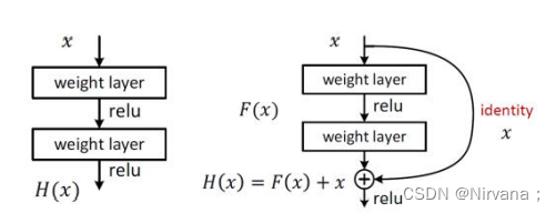
ResNet残差网络特点:
- 全是3X3卷积核
- 卷积步长2取代池化
- 使用BN
- 取消Max池化、全连接和Dropout
- 网络更深
各种ResNet残差网络: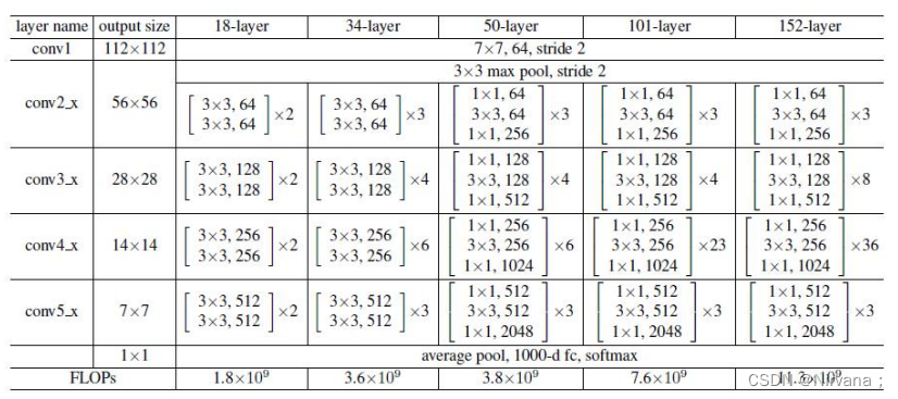
以Resnet18为例,它是由残差块堆叠而成的网络–1个卷积层+8个残差块(每个残差块有2个卷积层)+1个全连接层,如下图: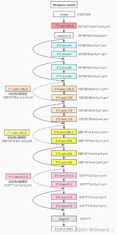
代码实现 ResNet18
#coding:utf-8import os
os.environ['TF_CPP_MIN_LOG_LEVEL']='2'import  tensorflow as tf
from    tensorflow import keras
from    tensorflow.keras import layers, Sequential

#构建残差块classBasicBlock(layers.Layer):def__init__(self, filter_num, stride=1):super(BasicBlock, self).__init__()#卷积层(过滤器尺寸3*3,过滤器个数filter_num(可变),步长为stride(可变),padding为same(输出尺寸=输入尺寸/步长)
        self.conv1 = layers.Conv2D(filter_num,(3,3), strides=stride, padding='same')#BatchNormalization标准化
        self.bn1 = layers.BatchNormalization()#激活函数选择relu
        self.relu = layers.Activation('relu')#卷积层(过滤器尺寸3*3,过滤器个数filter_num(可变),步长为1,padding为same(输出尺寸=输入尺寸/步长)
        self.conv2 = layers.Conv2D(filter_num,(3,3), strides=1, padding='same')
        self.bn2 = layers.BatchNormalization()#对步长进行判断,以减少参数量(如果步长等于1,则为原x;否则将x输入一个过滤器为1、步长为stride的卷积层中)if stride !=1:#建立一个容器
            self.downsample = Sequential()# 卷积层(过滤器尺寸1*1,过滤器个数filter_num(可变),步长为stride(可变));输出尺寸=向下取整((输入尺寸-过滤器尺寸)/步长)+1)
            self.downsample.add(layers.Conv2D(filter_num,(1,1), strides=stride))else:
            self.downsample =lambda x:x

    #前向传播defcall(self, inputs, training=None):# [b, h, w, c]
        out = self.conv1(inputs)
        out = self.bn1(out)
        out = self.relu(out)

        out = self.conv2(out)
        out = self.bn2(out)

        identity = self.downsample(inputs)

        output = layers.add([out, identity])
        output = tf.nn.relu(output)return output

#建立残差网络模型classResNet(keras.Model):#通过在__init__中定义层的实现def__init__(self, layer_dims, num_classes=100):#resnet18的layer_dims为[2, 2, 2, 2]super(ResNet, self).__init__()

        self.stem = Sequential([layers.Conv2D(64,(3,3), strides=(1,1)),
                                layers.BatchNormalization(),
                                layers.Activation('relu'),
                                layers.MaxPool2D(pool_size=(2,2), strides=(1,1), padding='same')])

        self.layer1 = self.build_resblock(64,  layer_dims[0])
        self.layer2 = self.build_resblock(128, layer_dims[1], stride=2)
        self.layer3 = self.build_resblock(256, layer_dims[2], stride=2)
        self.layer4 = self.build_resblock(512, layer_dims[3], stride=2)# output: [b, 512, h, w],#GlobalAveragePooling2D(是平均池化的一个特例,主要是用来解决全连接的问题)是将输入特征图的每一个通道求平均得到一个数值,它不需要指定pool_size和strides等参数。返回的tensor是[batch_size, channels],例如:128个9*9的feature map,对每个feature map取最大值直接得到一个128维的特征向量。
        self.avgpool = layers.GlobalAveragePooling2D()
        self.fc = layers.Dense(num_classes)#在call函数中实现前向过程defcall(self, inputs, training=None):

        x = self.stem(inputs)

        x = self.layer1(x)
        x = self.layer2(x)
        x = self.layer3(x)
        x = self.layer4(x)# [b, c]
        x = self.avgpool(x)# [b, 100]
        x = self.fc(x)return x

   #串联多个残差块defbuild_resblock(self, filter_num, blocks, stride=1):

        res_blocks = Sequential()# may down sample
        res_blocks.add(BasicBlock(filter_num, stride))for _ inrange(1, blocks):
            res_blocks.add(BasicBlock(filter_num, stride=1))return res_blocks

defresnet18():return ResNet([2,2,2,2])
总结
今天介绍了图像分类中各种CNN的迭代过程,网络越来越深,网络的复杂度也不断增加,但图像分类的准确度连年上升。下一节开始介绍另一大类研究方向–图像识别,包括各种各样新的网络结构和算法,敬请期待🚗
版权归原作者 Nirvana; 所有, 如有侵权,请联系我们删除。