通过遗传算法进行超参数调整和自动时间序列建模

在以前的文章中我们介绍过一些基于遗传算法的知识，本篇文章将使用遗传算法处理机器学习模型和时间序列数据。

超参数调整（TPOT ）

自动机器学习（Auto ML）通过自动化整个机器学习过程，帮我们找到最适合预测的模型，对于机器学习模型来说Auto ML可能更多的意味着超参数的调整和优化。

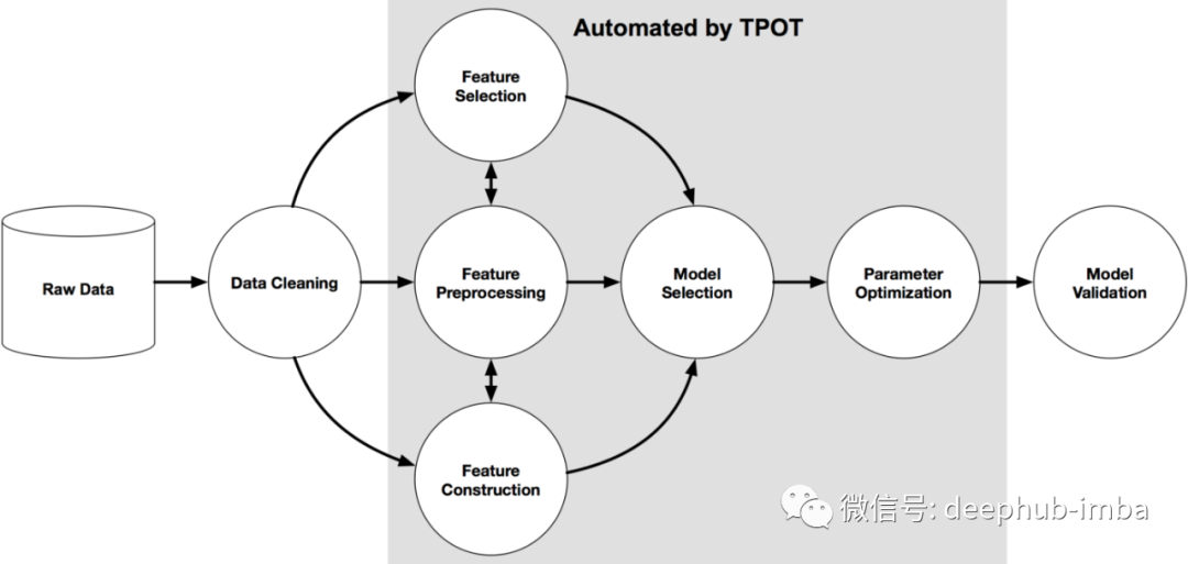
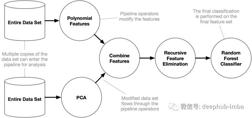
在这里我们使用python的一个名叫Tpot 的包来操作，TPOT 是建立在 scikit-learn 之上，虽然还是处在开发中，但是他的功能已经可以帮助我们了解这些概念了，下图显示了 Tpot 的工作原理：

from tpot import TPOTClassifier
from tpot import TPOTRegressormodel = TPOTClassifier(generations=100, population_size=100, offspring_size=None, mutation_rate=0.9, crossover_rate=0.1, scoring=None, cv=5, subsample=1.0, n_jobs=1, max_time_mins=None, max_eval_time_mins=5, random_state=None, config_dict=None, template=None, warm_start=False, memory=None, use_dask=False, periodic_checkpoint_folder=None, early_stop=None, verbosity=0, disable_update_check=False, log_file=None)

通过上面的代码就可以获得简单的回归模型，这是默认参数列表

generations=100, 
population_size=100, 
offspring_size=None  # Jeff notes this gets set to population_size
mutation_rate=0.9, 
crossover_rate=0.1, 
scoring="Accuracy",  # for Classification
cv=5, 
subsample=1.0, 
n_jobs=1,
max_time_mins=None, 
max_eval_time_mins=5,
random_state=None, 
config_dict=None,
warm_start=False, 
memory=None,
periodic_checkpoint_folder=None, 
early_stop=None
verbosity=0
disable_update_check=False

我们看看有哪些超参数可以进行调整：

generations ：迭代次数。默认值为 100。
population_size：每代遗传编程种群中保留的个体数。默认值为 100。
offspring_size：在每一代遗传编程中产生的后代数量。默认值为 100。
mutation_rate：遗传编程算法的突变率 范围[0.0, 1.0] 。该参数告诉 GP 算法有多少管道将随机更改应用于每词迭代。默认值为 0.9
crossover_rate：遗传编程算法交叉率， 范围[0.0, 1.0] 。这个参数告诉遗传编程算法每一代要“培育”多少管道。
scoring：用于评估问题函数，如准确率、平均精度、roc_auc、召回率等。默认为准确率。
cv：评估管道时使用的交叉验证策略。默认值为 5。
random_state：TPOT 中使用的伪随机数生成器的种子。使用此参数可确保运行 TPOT 时使用相同随机种子，得到相同的结果。
n_jobs：= -1多个 CPU 内核上运行以加快 tpot 进程。
period_checkpoint_folder：“any_string”，可以在训练分数提高的同时观察模型的演变。

mutation_rate + crossover_rate 不能超过 1.0。

下面我们将Tpot 和sklearn结合使用，进行模型的训练。

from pandas import read_csv
from sklearn.preprocessing import LabelEncoder
from sklearn.model_selection import RepeatedStratifiedKFold
from tpot import TPOTClassifier
dataframe = read_csv('sonar.csv')
#define X and y 
data = dataframe.values
X, y = data[:, :-1], data[:, -1]
# minimally prepare dataset
X = X.astype('float32')
y = LabelEncoder().fit_transform(y.astype('str'))
#split the dataset
from sklearn.model_selection import train_test_split
X_train, X_test, y_train, y_test = train_test_split(X, y, test_size = 0.2, random_state = 0)
# define cross validation 
cv = RepeatedStratifiedKFold(n_splits=10, n_repeats=3, random_state=1)

现在我们运行 TPOTClassifier，进行超参数的优化

#initialize the classifier
model = TPOTClassifier(generations=5, population_size=50,max_time_mins= 2,cv=cv, scoring='accuracy', verbosity=2, random_state=1, n_jobs=-1)
model.fit(X_train, y_train)
#export the best model
model.export('tpot_best_model.py')

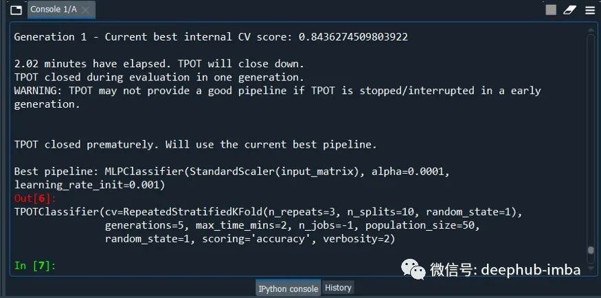
最后一句代码将模型保存在 .py 文件中，在使用的是后可以直接import。因为对于AutoML来说，最大的问题就是训练的时间，所以为了节省时间，population_size、max_time_mins 等值都使用了最小的设置。

现在我们打开文件 tpot_best_model.py，看看内容：

import numpy as np
import pandas as pd
from sklearn.linear_model import RidgeCV
from sklearn.model_selection import train_test_split
from sklearn.pipeline import make_pipeline
from sklearn.preprocessing import PolynomialFeatures
from tpot.export_utils import set_param_recursive
# NOTE: Make sure that the outcome column is labeled 'target' in the data file
tpot_data = pd.read_csv('PATH/TO/DATA/FILE', sep='COLUMN_SEPARATOR', dtype=np.float64)
features = tpot_data.drop('target', axis=1)
training_features, testing_features, training_target, testing_target = \
            train_test_split(features, tpot_data['target'], random_state=1)
# Average CV score on the training set was: -29.099695845082277
exported_pipeline = make_pipeline(
    PolynomialFeatures(degree=2, include_bias=False, interaction_only=False),
    RidgeCV()
)
# Fix random state for all the steps in exported pipeline
set_param_recursive(exported_pipeline.steps, 'random_state', 1)
exported_pipeline.fit(training_features, training_target)
results = exported_pipeline.predict(testing_features)

如果想做预测的话，使用下面代码

yhat = exported_pipeline.predict(new_data)

以上就是遗传算法进行AutoML/机器学习中超参数优化的方法。遗传算法受到达尔文自然选择过程的启发，并被用于计算机科学以寻找优化搜索。简而言之遗传算法由 3 种常见行为组成：选择、交叉、突变

下面我们看看它对处理时间序列的模型有什么帮助

时间序列数据建模（AutoTS）

在Python中有一个名叫 AutoTS 的包可以处理时间序列数据，我们从它开始

#AutoTS
from autots import AutoTS
from autots.models.model_list import model_lists
print(model_lists)

autots中有大量不同类型的时间序列模型，他就是以这些算法为基础，通过遗传算法的优化来找到最优的模型。

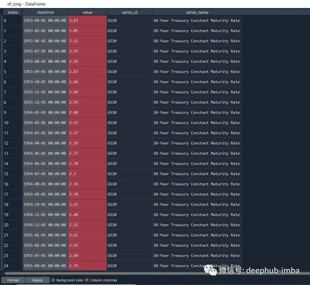
现在让我们加载数据。

#default data
from autots.datasets import load_monthly
#data was in long format
df_long = load_monthly(long=True)

用不同的参数初始化AutoTS

model = AutoTS(
    forecast_length=3,
    frequency='infer',
    ensemble='simple',
    max_generations=5,
    num_validations=2,
)
model = model.fit(df_long, date_col='datetime', value_col='value', id_col='series_id')
#help(AutoTS)

这个步骤需要很长的时间，因为它必须经过多次算法迭代。

print(model)

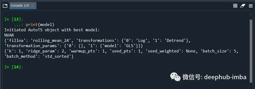
我们还可以查看模型准确率分数

#accuracy score
model.results()
#aggregated from cross validation
validation_results = model.results("validation")

从模型准确度分数列表中，还可以看到上面突出显示的“Ensemble”这一栏，它的低精度验证了一个理论，即Ensemble总是表现更好,这种说法是不正确的。

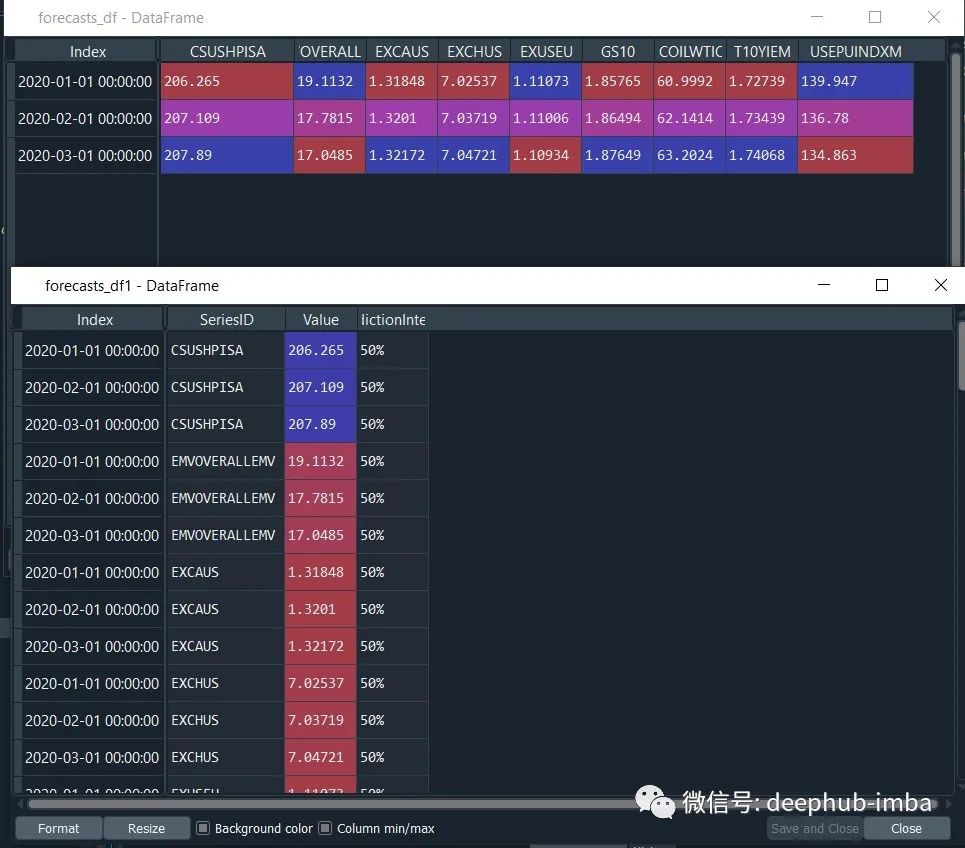
找到了最好的模型，就可以进行预测了。

prediction = model.predict()
forecasts_df = prediction.forecast
upper_forecasts_df = prediction.upper_forecast
lower_forecasts_df = prediction.lower_forecast
#or
forecasts_df1 = prediction.long_form_results()
upper_forecasts_df1 = prediction.long_form_results()
lower_forecasts_df1 = prediction.long_form_results()

默认的方法是使用AutoTs提供的所有模型进行训练，如果我们想要在一些模型列表上执行，并对某个特性设定不同的权重，就需要一些自定义的配置。

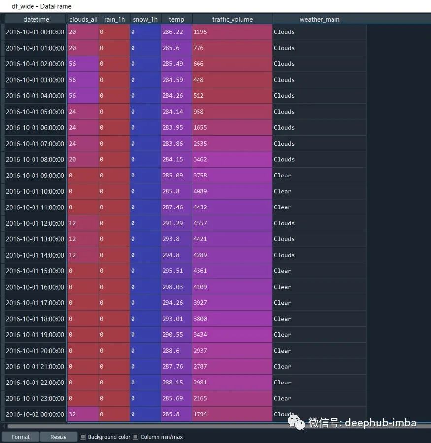
首先还是读取数据

from autots import AutoTS
from autots.datasets import load_hourlydf_wide = load_hourly(long=False)
# here we care most about traffic volume, all other series assumed to be weight of 1
weights_hourly = {'traffic_volume': 20}

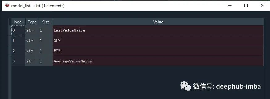
定义模型列表：

model_list = [
    'LastValueNaive',
    'GLS',
    'ETS',
    'AverageValueNaive',
]
model = AutoTS(
    forecast_length=49,
    frequency='infer',
    prediction_interval=0.95,
    ensemble=['simple', 'horizontal-min'],
    max_generations=5,
    num_validations=2,
    validation_method='seasonal 168',
    model_list=model_list,
    transformer_list='all',
    models_to_validate=0.2,
    drop_most_recent=1,
    n_jobs='auto',
)

在用数据拟合模型时定义权重：

model = model.fit(
    df_wide,
    weights=weights_hourly,
)
prediction = model.predict()
forecasts_df = prediction.forecast

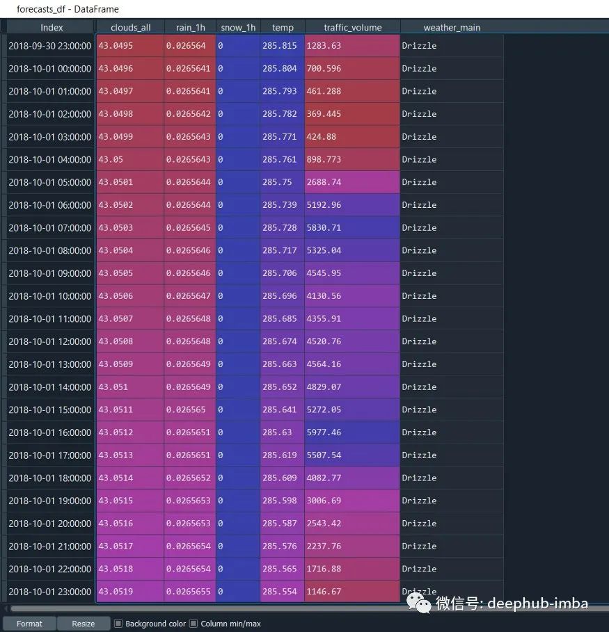
这样就完成了，对于使用来说非常的简单

通过遗传算法进行超参数调整和自动时间序列建模

超参数调整（TPOT ）

时间序列数据建模（AutoTS）

相关资源

发表评论

“通过遗传算法进行超参数调整和自动时间序列建模”的评论:

关于作者

Deephub

相关阅读

文章导航