mmsegmentation中可视化

samples_per_gpu=1,  ## 单个 GPU 的批量大小
workers_per_gpu=4,  ## 为每个 GPU 预取数据的 Worker 

1、tools/train.py

CUDA_VISIBLE_DEVICES=7指定固定的GPU，--work-dir表示configs保存的目录

CUDA_VISIBLE_DEVICES=7 python tools/train.py configs/seaformer/seaformer_base_512x512_160k_2x8_ade20k.py --work-dir result/seaformer/base16 

**tools/dist_train.sh **

该脚本是用于启动单机多卡/多机多卡分布式训练的，里面内容不多，无非是对

python -m torch.distributed.launch ...

的封装，留给用户的接口很简单，只需要指定想要用的 GPU 的个数即可，

bash tools/dist_train.sh configs/seaformer/seaformer_base_512x512_160k_2x8_ade20k.py --work-dir result/seaformer/base16  3

2、tools/test.py

输出可视化结果至目录文件夹

• 可以选择评估方式 --eval ，对于 COCO 数据集，可选 bbox 、segm、proposal ；对于 VOC 数据集，可选 map、recall
• 也可以选择 --out ，指定测试结果的 pkl 输出文件

python tools/test.py ${CONFIG_FILE} ${CHECKPOINT_FILE} [--out ${RESULT_FILE}] [--eval ${EVAL_METRICS}] [--show]

可视化具体实例如下：

#1、验证图像的可视化
python tools/test.py configs/fcn/fcn_r50-d8_512x512_20k_voc12.py work_dir/latest.pth --show-dir="output"
#或者
python tools/test.py configs/fcn/fcn_r50-d8_512x512_20k_voc12.py work_dir/latest.pth --show-dir output

#2、衡量指标显示
python tools/test.py configs/fcn/fcn_r50-d8_512x512_20k_voc12.py work_dir/latest.pth --eval mAp

• RESULT_FILE：输出结果的文件名，采用pickle格式。如果未指定，结果将不会保存到文件中。
• EVAL_METRICS：要根据结果评估的项目。允许的值是：COCO:proposal_fast, proposal, bbox, segm PASCAL VOC: mAP, recall
• --show：如果指定，检测结果将绘制在图像上并显示在新窗口中。仅适用于单GPU测试，用于调试和可视化。请确保您的环境中可以使用GUI，否则您可能会遇到类似的错误。cannot ``````connect ``````to ``````X ``````server
• --show-dir: 如果指定，检测结果将绘制在图像上并保存到指定的目录中。仅适用于单GPU测试，用于调试和可视化。使用此选项时，您的环境中不需要可用的GUI。
• --show-score-thr: 如果指定，则将删除分数低于此阈值的检测。

show-dir 参数来控制是否输出绘制的图像，表示输出图像的路径。

指定输出到 pkl 文件：

python tools/test.py configs/my_coco_config/my_coco_config.py checkpoints/faster_rcnn_r50_fpn_1x_coco_20200130-047c8118.pth  --out faster_rcnn_fpn_coco.pkl

3. 分析日志

pip install seaborn

python tools/analyze_logs.py plot_curve [--keys ${KEYS}] [--title ${TITLE}] [--legend ${LEGEND}] [--backend ${BACKEND}] [--style ${STYLE}] [--out ${OUT_FILE}]

• 绘制分类损失

• python tools/analyze_logs.py plot_curve log.json --keys loss_cls --legend loss_cls

• 日志分析：

• 用于分析我们训练过程中得到的日志文件，注意这里传入的日志文件必须是 json 文件，而第一个参数 plot_curve 有两个可选项：plot_curve 和 cal_train_time ，同样可以通过 --out 指定输出图片文件。
• 具体实例如下：
• python tools/analysis_tools/analyze_logs.py plot_curve work_dirs/my_coco_config/20220503_165551.log.json --out log_curve.png
• 
• 绘制训练时的分类和回归损失，并将该图保存为pdf。
• python tools/analyze_logs.py plot_curve log.json --keys loss_cls loss_bbox --out losses.pdf
• 在同一个图中绘制两次训练的bbox mAP
• python tools/analyze_logs.py plot_curve log1.json log2.json --keys bbox_mAP --legend run1 run2## 4、Flops、Params、fps的实现
• 本工具用于统计模型的参数量，可以通过 --shape 参数指定输入图片的尺寸
• python tools/get_flops.py ${CONFIG_FILE} [--shape ${INPUT_SHAPE}]例如：python tools/get_flops.py configs/danet/danet_r101-d8_512x512_20k_voc12aug.py#如果想在指定GPU上运行则执行以下代码 CUDA_VISIBLE_DEVICES=2 python tools/get_flops.py configs/danet/danet_r101-d8_512x512_20k_voc12aug.py python tools/analysis_tools/get_flops.py configs/my_coco_config/my_coco_config.py --shape 640 480输出结果为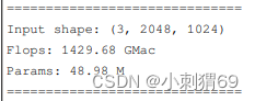 ## fps的实现：

• tools/benchmark.py 此工具是用来测试模型在当前环境下的推理速度的，模型会跑一遍配置文件中指定的测试集，计算单图推理时间（FPS）。

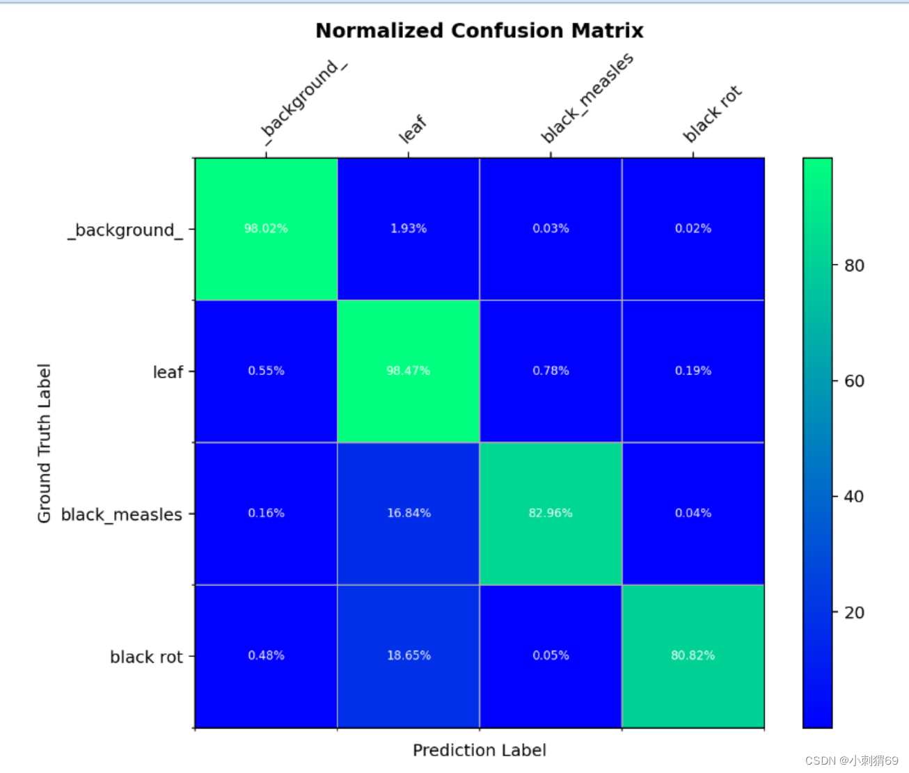
• CUDA_VISIBLE_DEVICES=4 python tools/benchmark.py configs/seaformer/seaformer_large_512x512_160k_2x8_ade20k.py result/seaformer/large16/iter_150000.pth## 5、混淆矩阵
• 计算混淆矩阵，需要输入的三个参数是：config文件，pkl结果文件，输出目录
• mkdir coco_confusion_matrix python tools/analysis_tools/confusion_matrix.py configs/my_coco_config/my_coco_config.py faster_rcnn_fpn_coco.pkl coco_confusion_matrix

• 6、画 PR 曲线 plot_pr_curve.py

• import osimport sysimport mmcvimport numpy as npimport argparseimport matplotlib.pyplot as pltfrom pycocotools.coco import COCOfrom pycocotools.cocoeval import COCOevalfrom mmcv import Configfrom mmdet.datasets import build_datasetdef plot_pr_curve(config_file, result_file, out_pic, metric="bbox"): """plot precison-recall curve based on testing results of pkl file. Args: config_file (list[list | tuple]): config file path. result_file (str): pkl file of testing results path. metric (str): Metrics to be evaluated. Options are 'bbox', 'segm'. """ cfg = Config.fromfile(config_file) # turn on test mode of dataset if isinstance(cfg.data.test, dict): cfg.data.test.test_mode = True elif isinstance(cfg.data.test, list): for ds_cfg in cfg.data.test: ds_cfg.test_mode = True # build dataset dataset = build_dataset(cfg.data.test) # load result file in pkl format pkl_results = mmcv.load(result_file) # convert pkl file (list[list | tuple | ndarray]) to json json_results, _ = dataset.format_results(pkl_results) # initialize COCO instance coco = COCO(annotation_file=cfg.data.test.ann_file) coco_gt = coco coco_dt = coco_gt.loadRes(json_results[metric]) # initialize COCOeval instance coco_eval = COCOeval(coco_gt, coco_dt, metric) coco_eval.evaluate() coco_eval.accumulate() coco_eval.summarize() # extract eval data precisions = coco_eval.eval["precision"] ''' precisions[T, R, K, A, M] T: iou thresholds [0.5 : 0.05 : 0.95], idx from 0 to 9 R: recall thresholds [0 : 0.01 : 1], idx from 0 to 100 K: category, idx from 0 to ... A: area range, (all, small, medium, large), idx from 0 to 3 M: max dets, (1, 10, 100), idx from 0 to 2 ''' pr_array1 = precisions[0, :, 0, 0, 2] pr_array2 = precisions[1, :, 0, 0, 2] pr_array3 = precisions[2, :, 0, 0, 2] pr_array4 = precisions[3, :, 0, 0, 2] pr_array5 = precisions[4, :, 0, 0, 2] pr_array6 = precisions[5, :, 0, 0, 2] pr_array7 = precisions[6, :, 0, 0, 2] pr_array8 = precisions[7, :, 0, 0, 2] pr_array9 = precisions[8, :, 0, 0, 2] pr_array10 = precisions[9, :, 0, 0, 2] x = np.arange(0.0, 1.01, 0.01) # plot PR curve plt.plot(x, pr_array1, label="iou=0.5") plt.plot(x, pr_array2, label="iou=0.55") plt.plot(x, pr_array3, label="iou=0.6") plt.plot(x, pr_array4, label="iou=0.65") plt.plot(x, pr_array5, label="iou=0.7") plt.plot(x, pr_array6, label="iou=0.75") plt.plot(x, pr_array7, label="iou=0.8") plt.plot(x, pr_array8, label="iou=0.85") plt.plot(x, pr_array9, label="iou=0.9") plt.plot(x, pr_array10, label="iou=0.95") plt.xlabel("recall") plt.ylabel("precison") plt.xlim(0, 1.0) plt.ylim(0, 1.01) plt.grid(True) plt.legend(loc="lower left") plt.savefig(out_pic)if __name__ == "__main__": parser = argparse.ArgumentParser() parser.add_argument('config', help='config file path') parser.add_argument('pkl_result_file', help='pkl result file path') parser.add_argument('--out', default='pr_curve.png') parser.add_argument('--eval', default='bbox') cfg = parser.parse_args() plot_pr_curve(config_file=cfg.config, result_file=cfg.pkl_result_file, out_pic=cfg.out, metric=cfg.eval)``````python plot_pr_curve.py configs/my_coco_config/my_coco_config.py faster_rcnn_fpn_coco.pkl这里用到的 pkl 结果文件，即是上面运行 tools/test.py 指定 --out 的输出文件。