HIVE高级调优（四）

1、Explain 查看执行计划

1.1、创建测试用表，数据准备

准备数据小表数据大表数据
建大表、小表和 JOIN 后表的语句

// 创建大表
create table bigtable(id bigint, t bigint, uid string, keyword string, url_rank int, click_num int, click_url string) row format delimited fields terminated by '\t';
// 创建小表
create table smalltable(id bigint, t bigint, uid string, keyword string, url_rank int, click_num int, click_url string) row format delimited fields terminated by '\t';
// 创建 JOIN 后表
create table jointable(id bigint, t bigint, uid string, keyword string, url_rank int, click_num int, click_url string) row format delimited fields terminated by '\t';

分别向大表和小表中导入数据

hive (default)> load data local inpath '/opt/module/data/bigtable' into  table bigtable;
hive (default)> load data local inpath '/opt/module/data/smalltable' into table smalltable;

1.2、基本语法

EXPLAIN [EXTENDED | DEPENDENCY | AUTHORIZATION] query-sql

1.3、案例实操

查看下面这条语句的执行计划

hive (default)> explain select * from bigtable;
hive (default)> explain select click_url, count(*) ct from bigtable group by click_url;

查看详细执行计划

hive (default)> explain extended select * from bigtable;
hive (default)> explain extended select click_url, count(*) ct from bigtable group by click_url;

2、Hive 建表优化

2.1、分区表

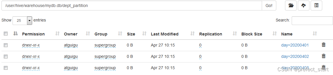
分区表实际上就是对应一个 HDFS 文件系统上的独立的文件夹，该文件夹下是该分区所有的数据文件。
Hive 中的分区就是分目录，把一个大的数据集根据业务需要分割成小的数据集。在查询时通过 WHERE 子句中的表达式选择查询所需要的指定的分区，这样的查询效率会提高很多，所以我们需要把常常用在 WHERE 语句中的字段指定为表的分区字段。

2.1.1、分区表基本操作

引入分区表（需要根据日期对日志进行管理, 通过部门信息模拟）

dept_20200401.log
dept_20200402.log
dept_20200403.log

创建分区表语法

hive (default)> create table dept_partition(
deptno int, dname string, loc string
)
partitioned by (day string) 
row format delimited fields terminated by '\t';

注意：分区字段不能是表中已经存在的数据，可以将分区字段看作表的伪列。

加载数据到分区表中

数据划分 dept_20200401.log

10 ACCOUNTING 1700
20 RESEARCH 1800

dept_20200402.log

30 SALES 1900
40 OPERATIONS 1700

dept_20200403.log

50 TEST 2000
60 DEV 1900

加载数据

hive (default)> load data local inpath '/opt/module/data/dept_20200401.log' into table dept_partition partition(day='20200401');
hive (default)> load data local inpath '/opt/module/data/dept_20200402.log' into table dept_partition partition(day='20200402');
hive (default)> load data local inpath '/opt/module/data/dept_20200403.log' into table dept_partition partition(day='20200403');

注意：分区表加载数据时，必须指定分区

在这里插入图片描述

查询分区表中数据

单分区查询

hive (default)> select * from dept_partition where day='20200401';

多分区联合查询

hive (default)> select * from dept_partition where day='20200401'  
 union 
 select * from dept_partition where day='20200402'   
 union
 select * from dept_partition where day='20200403';
hive (default)> select * from dept_partition where day='20200401' or  day='20200402' or day='20200403';

增加分区

增加单个分区

hive (default)> alter table dept_partition add partition(day='20200404');

同时增加多个分区

hive (default)> alter table dept_partition add partition(day='20200405')  partition(day='20200406');

删除分区

删除单个分区

hive (default)> alter table dept_partition drop partition  (day='20200406');

同时删除多个分区

hive (default)> alter table dept_partition drop partition  (day='20200404'), partition(day='20200405');

查看分区表有多少分区

hive> show partitions dept_partition;

查看分区表结构

hive> desc formatted dept_partition;
# Partition Information
# col_name data_type comment
month string

2.1.2、二级分区

如果当一天的日志数据量也很大，可以将数据再次拆分

创建二级分区表

hive (default)> create table dept_partition2(
    deptno int, 
    dname string, 
    loc string
)
partitioned by (day string, hour string) row format delimited fields terminated by '\t';

正常的加载数据

加载数据到二级分区表中

hive (default)> load data local inpath '/opt/module/data/dept_20200401.log' into table dept_partition2 partition(day='20200401', hour='12');

查询分区数据

hive (default)> select * from dept_partition2 where day='20200401' and  hour='12';

2.1.3、动态分区

关系型数据库中，对分区表 Insert 数据时候，数据库自动会根据分区字段的值，将数据插入到相应的分区中，Hive 中也提供了类似的机制，即动态分区(Dynamic Partition)，只不过，使用 Hive 的动态分区，需要进行相应的配置。

开启动态分区参数设置

开启动态分区功能（默认 true，开启）

set hive.exec.dynamic.partition=true;

设置为非严格模式（动态分区的模式，默认 strict，表示必须指定至少一个分区为静态分区，nonstrict 模式表示允许所有的分区字段都可以使用动态分区。）

set hive.exec.dynamic.partition.mode=nonstrict;

在所有执行 MR 的节点上，最大一共可以创建多少个动态分区。默认 1000

set hive.exec.max.dynamic.partitions=1000;

在每个执行 MR 的节点上，最大可以创建多少个动态分区。该参数需要根据实际的数据来设定。比如：源数据中包含了一年的数据，即 day 字段有365 个值，那么该参数就需要设置成大于 365，如果使用默认值 100，则会报错。
整个 MR Job 中，最大可以创建多少个 HDFS 文件。默认 100000

set hive.exec.max.created.files=100000

当有空分区生成时，是否抛出异常。一般不需要设置。默认 false

set hive.error.on.empty.partition=false

案例实操，需求：将 dept 表中的数据按照地区（loc 字段），插入到目标表 dept_partition 的相应分区中。

创建目标分区表

hive (default)> create table dept_partition_dy(id int, name string) 
partitioned by (loc int) 
row format delimited fields terminated by '\t';

设置动态分区

hive (default)> set hive.exec.dynamic.partition.mode = nonstrict;
hive (default)> insert into table dept_partition_dy partition(loc) select deptno, dname, loc from dept;

查看目标分区表的分区情况

hive (default)> show partitions dept_partition;

2.2、分桶表

分区提供一个隔离数据和优化查询的便利方式。不过，并非所有的数据集都可形成合理的分区。对于一张表或者分区，Hive 可以进一步组织成桶，也就是更为细粒度的数据范围划分。
分桶是将数据集分解成更容易管理的若干部分的另一个技术。分区针对的是数据的存储路径，分桶针对的是数据文件。

2.2.1、创建分桶表

数据准备

1001 ss1
1002 ss2
1003 ss3
1004 ss4
1005 ss5
1006 ss6
1007 ss7
1008 ss8
1009 ss9
1010 ss10
1011 ss11
1012 ss12
1013 ss13
1014 ss14
1015 ss15
1016 ss16

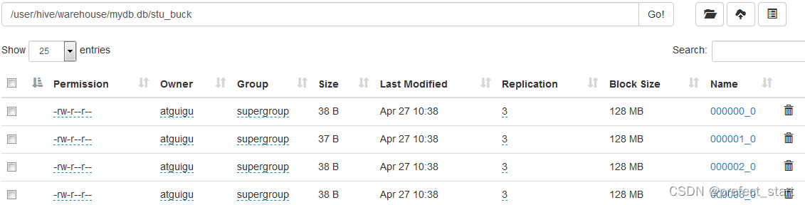
创建分桶表

create table stu_buck(id int, name string)
clustered by(id) 
into 4 buckets
row format delimited fields terminated by '\t';

查看表结构

hive (default)> desc formatted stu_buck;
Num Buckets: 4

导入数据到分桶表中，load 的方式

hive (default)> load data inpath '/student.txt' into table stu_buck;

查看创建的分桶表中是否分成 4 个桶
查询分桶的数据

hive(default)> select * from stu_buck;

分桶规则：根据结果可知：Hive 的分桶采用对分桶字段的值进行哈希，然后除以桶的个数求余的方式决定该条记录存放在哪个桶当中.
分桶表操作需要注意的事项:

reduce 的个数设置为-1，让 Job 自行决定需要用多少个 reduce 或者将 reduce 的个数设置为大于等于分桶表的桶数
从 hdfs 中 load 数据到分桶表中，避免本地文件找不到问题
不要使用本地模式

insert 方式将数据导入分桶表

hive(default)>insert into table stu_buck select * from student_insert;

2.2.2、抽样查询

对于非常大的数据集，有时用户需要使用的是一个具有代表性的查询结果而不是全部结果。Hive 可以通过对表进行抽样来满足这个需求。
语法: TABLESAMPLE(BUCKET x OUT OF y)
查询表 stu_buck 中的数据。

hive (default)> select * from stu_buck tablesample(bucket 1 out of 4 on id);

注意：x 的值必须小于等于 y 的值，否则报错

FAILED: SemanticException [Error 10061]: Numerator should not be bigger than denominator in sample clause for table stu_buck

2.3、合适的存储文件格式

Hive 支持的存储数据的格式主要有：TEXTFILE 、SEQUENCEFILE、ORC、PARQUET。

2.3.1、列式存储和行式存储

在这里插入图片描述
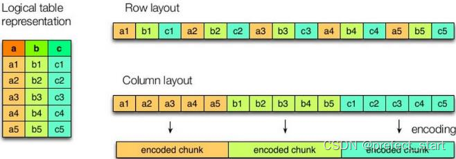
如图所示左边为逻辑表，右边第一个为行式存储，第二个为列式存储。

行存储的特点查询满足条件的一整行数据的时候，列存储则需要去每个聚集的字段找到对应的每个列的值，行存储只需要找到其中一个值，其余的值都在相邻地方，所以此时行存储查询的速度更快。
列存储的特点因为每个字段的数据聚集存储，在查询只需要少数几个字段的时候，能大大减少读取的数据量；每个字段的数据类型一定是相同的，列式存储可以针对性的设计更好的设计压缩算法。 TEXTFILE 和 SEQUENCEFILE 的存储格式都是基于行存储的； ORC 和 PARQUET 是基于列式存储的。

2.3.2、TextFile 格式

默认格式，数据不做压缩，磁盘开销大，数据解析开销大。可结合 Gzip、Bzip2 使用，但使用 Gzip 这种方式，hive 不会对数据进行切分，从而无法对数据进行并行操作。

2.3.3、Orc 格式

Orc (Optimized Row Columnar)是 Hive 0.11 版里引入的新的存储格式。

2.3.4、 Parquet 格式

Parquet 文件是以二进制方式存储的，所以是不可以直接读取的，文件中包括该文件的数据和元数据，因此 Parquet 格式文件是自解析的

2.4、合适的压缩格式

在这里插入图片描述
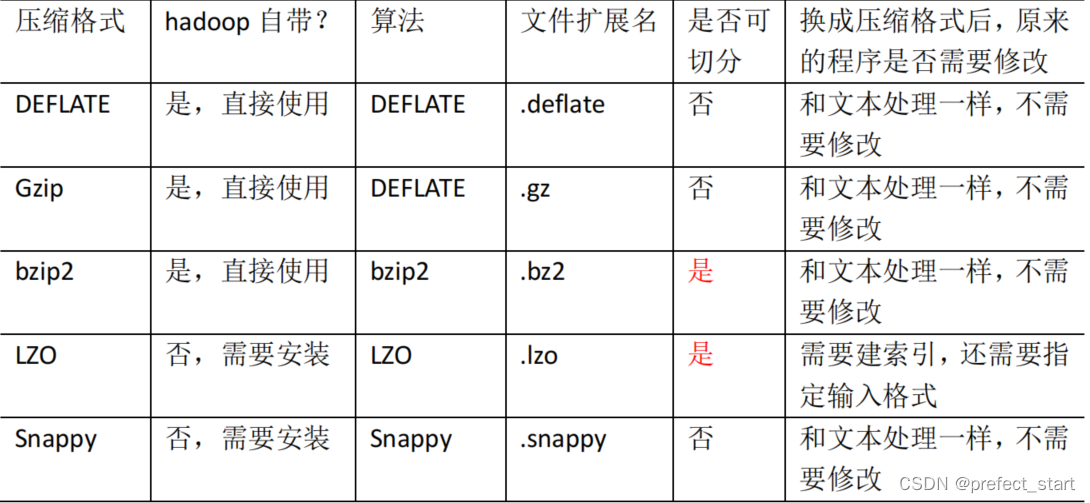
压缩格式对应的编码/解码器DEFLATEorg.apache.hadoop.io.compress.DefaultCodecgziporg.apache.hadoop.io.compress.GzipCodecbzip2org.apache.hadoop.io.compress.BZip2CodecLZOcom.hadoop.compression.lzo.LzopCodecSnappyorg.apache.hadoop.io.compress.SnappyCodec
压缩性能的比较：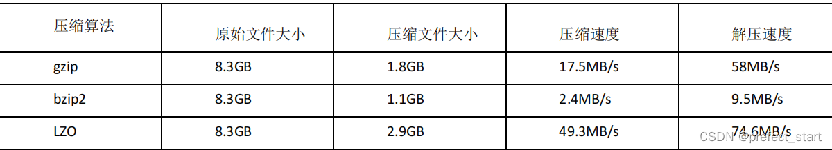
在这里插入图片描述
更多了解

3、HQL 语法优化

3.1、列裁剪与分区裁剪

列裁剪就是在查询时只读取需要的列，分区裁剪就是只读取需要的分区。当列很多或者数据量很大时，如果 select * 或者不指定分区，全列扫描和全表扫描效率都很低。
Hive 在读数据的时候，可以只读取查询中所需要用到的列，而忽略其他的列。这样做可以节省读取开销：中间表存储开销和数据整合开销。

3.2、Group By

默认情况下，Map 阶段同一 Key 数据分发给一个 Reduce，当一个 key 数据过大时就倾斜了。

在这里插入图片描述
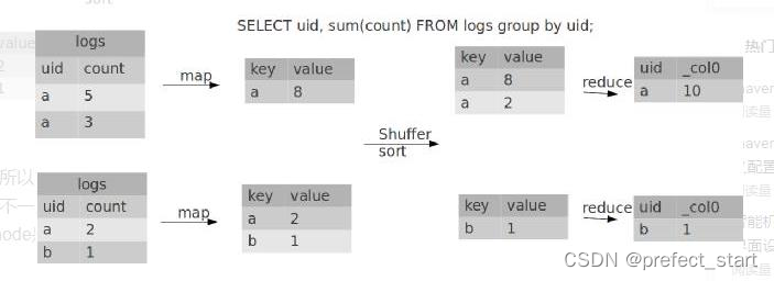
并不是所有的聚合操作都需要在 Reduce 端完成，很多聚合操作都可以先在 Map 端进行部分聚合，最后在 Reduce 端得出最终结果。

开启 Map 端聚合参数设置

是否在 Map 端进行聚合，默认为 True

set hive.map.aggr = true;

在 Map 端进行聚合操作的条目数目

set hive.groupby.mapaggr.checkinterval = 100000;

有数据倾斜的时候进行负载均衡（默认是 false）

set hive.groupby.skewindata = true;

当选项设定为 true，生成的查询计划会有两个 MR Job。

第一个 MR Job 中，Map 的输出结果会随机分布到 Reduce 中，每个 Reduce 做部分聚合操作，并输出结果，这样处理的结果是相同的 Group By Key 有可能被分发到不同的 Reduce中，从而达到负载均衡的目的；
第二个 MR Job 再根据预处理的数据结果按照 Group By Key 分布到 Reduce 中（这个过程可以保证相同的 Group By Key 被分布到同一个 Reduce 中），最后完成最终的聚合操作（虽然能解决数据倾斜，但是不能让运行速度的更快）。

hive (default)> select deptno from emp group by deptno;
Stage-Stage-1: Map: 1 Reduce: 5 Cumulative CPU: 23.68 sec HDFS Read: 
19987 HDFS Write: 9 SUCCESS
Total MapReduce CPU Time Spent: 23 seconds 680 msec
OK
deptno
10
20
30

优化以后

hive (default)> set hive.groupby.skewindata = true;
hive (default)> select deptno from emp group by deptno;
Stage-Stage-1: Map: 1 Reduce: 5 Cumulative CPU: 28.53 sec HDFS Read: 
18209 HDFS Write: 534 SUCCESS
Stage-Stage-2: Map: 1 Reduce: 5 Cumulative CPU: 38.32 sec HDFS Read: 
15014 HDFS Write: 9 SUCCESS
Total MapReduce CPU Time Spent: 1 minutes 6 seconds 850 msec
OK
deptno
10
20
30

3.3、Vectorization

vectorization : 矢量计算的技术，在计算类似scan, filter, aggregation的时候，vectorization技术以设置批处理的增量大小为 1024 行单次来达到比单条记录单次获得更高的效率。

在这里插入图片描述

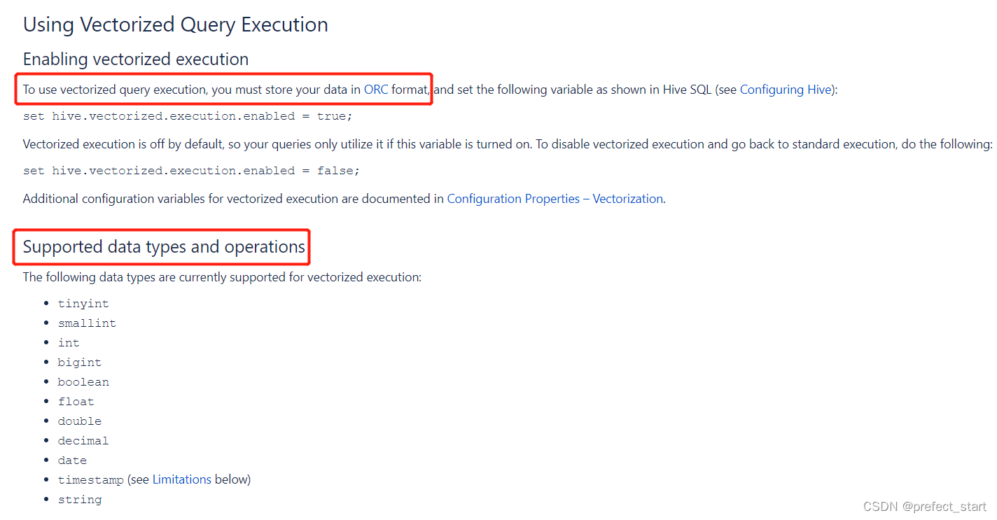
set hive.vectorized.execution.enabled = true;
set hive.vectorized.execution.reduce.enabled = true;

3.4、多重模式

如果你碰到一堆 SQL，并且这一堆 SQL 的模式还一样。都是从同一个表进行扫描，做不同的逻辑。有可优化的地方：如果有 n 条 SQL，每个 SQL 执行都会扫描一次这张表。

insert .... select id,name,sex, age from student where age > 17;
insert .... select id,name,sex, age from student where age > 18;
insert .... select id,name,sex, age from student where age > 19;

就出现了一个问题：这种类型的 SQL 有多少个，那么最终。这张表就被全表扫描了多少次

insert int t_ptn partition(city=A). select id,name,sex, age from student where city= A;
insert int t_ptn partition(city=B). select id,name,sex, age from student where city= B;
insert int t_ptn partition(city=c). select id,name,sex, age from student where city= c;
修改为：
from student
insert int t_ptn partition(city=A) select id,name,sex, age where city= A
insert int t_ptn partition(city=B) select id,name,sex, age where city= B

如果一个 HQL 底层要执行 10 个 Job，那么能优化成 8 个一般来说，肯定能有所提高，多重插入就是一个非常实用的技能。一次读取，多次插入，有些场景是从一张表读取数据后，要多次利用。

3.5、in/exists 语句

在 Hive 的早期版本中，in/exists 语法是不被支持的，但是从 hive-0.8x 以后就开始支持这个语法。但是不推荐使用这个语法。虽然经过测验，Hive-2.3.6 也支持 in/exists 操作，但还是推荐使用 Hive 的一个高效替代方案：left semi join

比如说：-- in / exists 实现

select a.id, a.name from a where a.id in (select b.id from b);
select a.id, a.name from a where exists (select id from b where a.id = b.id);

可以使用 join 来改写：

select a.id, a.name from a join b on a.id = b.id;

应该转换成：
– left semi join 实现

select a.id, a.name from a left semi join b on a.id = b.id;

3.6、CBO 优化

join 的时候表的顺序的关系：前面的表都会被加载到内存中。后面的表进行磁盘扫描

select a.*, b.*, c.* from a join b on a.id = b.id join c on a.id = c.id;

Hive 自 0.14.0 开始，加入了一项 “Cost Based Optimizer” 来对 HQL 执行计划进行优化，这个功能通过 “hive.cbo.enable” 来开启。在 Hive 1.1.0 之后，这个 feature 是默认开启的，它可以自动优化 HQL 中多个 Join 的顺序，并选择合适的 Join 算法。

CBO，成本优化器，代价最小的执行计划就是最好的执行计划。传统的数据库，成本优化器做出最优化的执行计划是依据统计信息来计算的。

Hive 的成本优化器也一样，Hive 在提供最终执行前，优化每个查询的执行逻辑和物理执行计划。这些优化工作是交给底层来完成的。根据查询成本执行进一步的优化，从而产生潜在的不同决策：如何排序连接，执行哪种类型的连接，并行度等等。

要使用基于成本的优化（也称为 CBO），请在查询开始设置以下参数：

set hive.cbo.enable=true;
set hive.compute.query.using.stats=true;
set hive.stats.fetch.column.stats=true;
set hive.stats.fetch.partition.stats=true;

3.7、谓词下推

将 SQL 语句中的 where 谓词逻辑都尽可能提前执行，减少下游处理的数据量。对应逻辑优化器是 PredicatePushDown，配置项为 hive.optimize.ppd，默认为 true。

案例实操：

打开谓词下推优化属性

hive (default)> set hive.optimize.ppd = true; #谓词下推，默认是 true

查看先关联两张表，再用 where 条件过滤的执行计划

hive (default)> explain select o.id from bigtable b join bigtable o on o.id = b.id where o.id <= 10;

查看子查询后，再关联表的执行计划

hive (default)> explain select b.id from bigtable b join (select id from bigtable where id <= 10) o on b.id = o.id;

3.8、MapJoin

MapJoin 是将 Join 双方比较小的表直接分发到各个 Map 进程的内存中，在 Map 进程中进行 Join 操作，这样就不用进行 Reduce 步骤，从而提高了速度。如果不指定 MapJoin或者不符合 MapJoin 的条件，那么 Hive 解析器会将 Join 操作转换成 Common Join，即：在
Reduce 阶段完成 Join。容易发生数据倾斜。可以用 MapJoin 把小表全部加载到内存在 Map端进行 Join，避免 Reducer 处理。

开启 MapJoin 参数设置

设置自动选择 MapJoin

set hive.auto.convert.join=true; #默认为 true

大表小表的阈值设置（默认 25M 以下认为是小表）：

set hive.mapjoin.smalltable.filesize=25000000;

MapJoin 工作机制 MapJoin 是将 Join 双方比较小的表直接分发到各个 Map 进程的内存中，在 Map 进程中进行 Join 操作，这样就不用进行 Reduce 步骤，从而提高了速度。
案例实操：

开启 MapJoin 功能

set hive.auto.convert.join = true; 默认为 true

执行小表 JOIN 大表语句注意：此时小表(左连接)作为主表，所有数据都要写出去，因此此时会走 reduce，mapjoin 失效

Explain insert overwrite table jointable
select b.id, b.t, b.uid, b.keyword, b.url_rank, b.click_num, b.click_url
from smalltable s
left join bigtable b
on s.id = b.id;

Time taken: 24.594 seconds

执行大表 JOIN 小表语句

Explain insert overwrite table jointable
select b.id, b.t, b.uid, b.keyword, b.url_rank, b.click_num, b.click_url
from bigtable b
left join smalltable s
on s.id = b.id;

Time taken: 24.315 seconds

3.9、大表、大表 SMB Join（重点）

SMB Join ：Sort Merge Bucket Join

创建第二张大表

create table bigtable2(
 id bigint,
 t bigint,
 uid string,
 keyword string,
 url_rank int,
 click_num int,
 click_url string)
row format delimited fields terminated by '\t';
load data local inpath '/opt/module/data/bigtable' into table bigtable2;

测试大表直接 JOIN

insert overwrite table jointable
select b.id, b.t, b.uid, b.keyword, b.url_rank, b.click_num, b.click_url
from bigtable a
join bigtable2 b
on a.id = b.id;

测试结果：Time taken: 72.289 seconds

insert overwrite table jointable
select b.id, b.t, b.uid, b.keyword, b.url_rank, b.click_num, b.click_url
from bigtable a
join bigtable2 b
on a.id = b.id;

创建分通表 1

create table bigtable_buck1(
 id bigint,
 t bigint,
 uid string,
 keyword string,
 url_rank int,
 click_num int,
 click_url string)
clustered by(id)
sorted by(id)
into 6 buckets
row format delimited fields terminated by '\t';
load data local inpath '/opt/module/data/bigtable' into table bigtable_buck1;

4）创建分通表 2，分桶数和第一张表的分桶数为倍数关系

create table bigtable_buck2(
 id bigint,
 t bigint,
 uid string,
 keyword string,
 url_rank int,
 click_num int,
 click_url string)
clustered by(id)
sorted by(id)
into 6 buckets
row format delimited fields terminated by '\t';
load data local inpath '/opt/module/data/bigtable' into table bigtable_buck2;

设置参数

set hive.optimize.bucketmapjoin = true;
set hive.optimize.bucketmapjoin.sortedmerge = true;
set hive.input.format=org.apache.hadoop.hive.ql.io.BucketizedHiveInputFormat;

测试 Time taken: 34.685 seconds

insert overwrite table jointable
select b.id, b.t, b.uid, b.keyword, b.url_rank, b.click_num, b.click_url
from bigtable_buck1 s
join bigtable_buck2 b
on b.id = s.id;

3.10、笛卡尔积

Join 的时候不加 on 条件，或者无效的 on 条件，因为找不到 Join key，Hive 只能使用 1 个 Reducer 来完成笛卡尔积。当 Hive 设定为严格模式（hive.mapred.mode=strict，nonstrict）时，不允许在 HQL 语句中出现笛卡尔积。

4、数据倾斜

绝大部分任务都很快完成，只有一个或者少数几个任务执行的很慢甚至最终执行失败，这样的现象为数据倾斜现象。

一定要和数据过量导致的现象区分开，数据过量的表现为所有任务都执行的很慢，这个时候只有提高执行资源才可以优化 HQL 的执行效率。

综合来看，导致数据倾斜的原因在于按照 Key 分组以后，少量的任务负责绝大部分数据的计算，也就是说产生数据倾斜的 HQL 中一定存在分组操作，那么从 HQL 的角度，我们可以将数据倾斜分为单表携带了 GroupBy 字段的查询和两表（或者多表）Join 的查询。

4.1、单表数据倾斜优化

4.1.1、使用参数

当任务中存在 GroupBy 操作同时聚合函数为 count 或者 sum 可以设置参数来处理数据倾斜问题。

是否在 Map 端进行聚合，默认为 True

set hive.map.aggr = true;

在 Map 端进行聚合操作的条目数目

set hive.groupby.mapaggr.checkinterval = 100000;

有数据倾斜的时候进行负载均衡（默认是 false）

set hive.groupby.skewindata = true;

当选项设定为 true，生成的查询计划会有两个 MR Job。

4.1.2、增加 Reduce 数量（多个 Key 同时导致数据倾斜）

调整 reduce 个数方法一

每个 Reduce 处理的数据量默认是 256MB

set hive.exec.reducers.bytes.per.reducer = 256000000

每个任务最大的 reduce 数，默认为 1009

set hive.exec.reducers.max = 1009

计算 reducer 数的公式

N=min(参数 2，总输入数据量/参数 1)(参数 2 指的是上面的 1009，参数 1 值得是 256M)

调整 reduce 个数方法二在 hadoop 的 mapred-default.xml 文件中修改，设置每个 job 的 Reduce 个数

set mapreduce.job.reduces = 15;

4.2、Join 数据倾斜优化

4.2.1、使用参数

在编写 Join 查询语句时，如果确定是由于 join 出现的数据倾斜，那么请做如下设置：
# join 的键对应的记录条数超过这个值则会进行分拆，值根据具体数据量设置
set hive.skewjoin.key=100000;
# 如果是 join 过程出现倾斜应该设置为 true
set hive.optimize.skewjoin=false;

如果开启了，在 Join 过程中 Hive 会将计数超过阈值

hive.skewjoin.key（默认 100000）

的倾斜 key 对应的行临时写进文件中，然后再启动另一个 job 做 map join 生成结果。通过

hive.skewjoin.mapjoin.map.tasks

参数还可以控制第二个 job 的 mapper 数量，默认 10000。

set hive.skewjoin.mapjoin.map.tasks=10000;

5、Hive Job 优化

5.1、Hive Map 优化

5.1.1、复杂文件增加 Map 数

当 input 的文件都很大，任务逻辑复杂，map 执行非常慢的时候，可以考虑增加 Map 数，来使得每个 map 处理的数据量减少，从而提高任务的执行效率。
增加 map 的方法为：
根据

computeSliteSize(Math.max(minSize,Math.min(maxSize,blocksize)))=blocksize=128M

公式，调整 maxSize 最大值。让 maxSize 最大值低于 blocksize 就可以增加 map 的个数。

执行查询

hive (default)> select count(*) from emp;
Hadoop job information for Stage-1: number of mappers: 1; number of 
reducers: 1

设置最大切片值为 100 个字节

hive (default)> set mapreduce.input.fileinputformat.split.maxsize=100;
hive (default)> select count(*) from emp;
Hadoop job information for Stage-1: number of mappers: 6; number of 
reducers: 1

5.1.2、小文件进行合并

在 map 执行前合并小文件，减少 map 数：CombineHiveInputFormat 具有对小文件进行合并的功能（系统默认的格式）。HiveInputFormat 没有对小文件合并功能。

set hive.input.format= org.apache.hadoop.hive.ql.io.CombineHiveInputFormat;

在 Map-Reduce 的任务结束时合并小文件的设置：

在 map-only 任务结束时合并小文件，默认 true

set hive.merge.mapfiles = true;

在 map-reduce 任务结束时合并小文件，默认 false

set hive.merge.mapredfiles = true;

合并文件的大小，默认 256M

set hive.merge.size.per.task = 268435456;

当输出文件的平均大小小于该值时，启动一个独立的 map-reduce 任务进行文件 merge

set hive.merge.smallfiles.avgsize = 16777216;

5.1.3、Map 端聚合

set hive.map.aggr=true;相当于 map 端执行 combiner

5.1.4、推测执行

set mapred.map.tasks.speculative.execution = true #默认是 true

5.2、Hive Reduce 优化

5.2.1、合理设置 Reduce 数

调整 reduce 个数方法一

每个 Reduce 处理的数据量默认是 256MB

set hive.exec.reducers.bytes.per.reducer = 256000000

每个任务最大的 reduce 数，默认为 1009

set hive.exec.reducers.max = 1009

计算 reducer 数的公式

N=min(参数 2，总输入数据量/参数 1)(参数 2 指的是上面的 1009，参数 1 值得是 256M)

调整 reduce 个数方法二

在 hadoop 的 mapred-default.xml 文件中修改，设置每个 job 的 Reduce 个数

set mapreduce.job.reduces = 15;

reduce 个数并不是越多越好

过多的启动和初始化 reduce 也会消耗时间和资源；
另外，有多少个 reduce，就会有多少个输出文件，如果生成了很多个小文件，那么如果这些小文件作为下一个任务的输入，则也会出现小文件过多的问题；
在设置 reduce 个数的时候也需要考虑这两个原则：处理大数据量利用合适的 reduce 数；使单个 reduce 任务处理数据量大小要合适；

5.2.2、推测执行

mapred.reduce.tasks.speculative.execution （hadoop 里面的）
hive.mapred.reduce.tasks.speculative.execution（hive 里面相同的参数，效果和hadoop 里面的一样两个随便哪个都行）

5.3、Hive 任务整体优化

5.3.1、Fetch 抓取

Fetch 抓取是指，Hive 中对某些情况的查询可以不必使用 MapReduce 计算。例如

：SELECT * FROM emp;

在这种情况下，Hive 可以简单地读取 emp 对应的存储目录下的文件，然后输出查询结果到控制台。

在 hive-default.xml.template 文件中

hive.fetch.task.conversion 默认是 more

，老版本 hive默认是 minimal，该属性修改为 more 以后，在全局查找、字段查找、limit 查找等都不走mapreduce。

<property><name>hive.fetch.task.conversion</name><value>more</value><description>
 Expects one of [none, minimal, more].
 Some select queries can be converted to single FETCH task minimizing latency.
 Currently the query should be single sourced not having any subquery and should not have any aggregations or distincts (which incurs RS), 
lateral views and joins.
 0. none : disable hive.fetch.task.conversion
 1. minimal : SELECT STAR, FILTER on partition columns, LIMIT only
 2. more : SELECT, FILTER, LIMIT only (support TABLESAMPLE and 
virtual columns)
 </description></property>

案例实操：

把 hive.fetch.task.conversion 设置成 none，然后执行查询语句，都会执行 mapreduce程序。

hive (default)> set hive.fetch.task.conversion=none;
hive (default)> select * from emp;
hive (default)> select ename from emp;
hive (default)> select ename from emp limit 3;

把 hive.fetch.task.conversion 设置成 more，然后执行查询语句，如下查询方式都不会执行 mapreduce 程序。

hive (default)> set hive.fetch.task.conversion=more;
hive (default)> select * from emp;
hive (default)> select ename from emp;
hive (default)> select ename from emp limit 3;

5.3.2、本地模式

大多数的 Hadoop Job 是需要 Hadoop 提供的完整的可扩展性来处理大数据集的。不过，有时 Hive 的输入数据量是非常小的。在这种情况下，为查询触发执行任务消耗的时间可能会比实际 job 的执行时间要多的多。对于大多数这种情况，Hive 可以通过本地模式在单台机器上处理所有的任务。对于小数据集，执行时间可以明显被缩短。

用户可以通过设置

hive.exec.mode.local.auto 的值为 true

，来让 Hive 在适当的时候自动启动这个优化。

set hive.exec.mode.local.auto=true; //开启本地 mr
//设置 local mr 的最大输入数据量，当输入数据量小于这个值时采用 local mr 的方式，默认为 134217728，即 128M
set hive.exec.mode.local.auto.inputbytes.max=50000000;
//设置 local mr 的最大输入文件个数，当输入文件个数小于这个值时采用 local mr 的方式，默认为 4
set hive.exec.mode.local.auto.input.files.max=10;

案例实操：

开启本地模式，并执行查询语句

hive (default)> set hive.exec.mode.local.auto=true;
hive (default)> select * from emp cluster by deptno;
Time taken: 1.328 seconds, Fetched: 14 row(s)

关闭本地模式，并执行查询语句

hive (default)> set hive.exec.mode.local.auto=false;
hive (default)> select * from emp cluster by deptno;
Time taken: 20.09 seconds, Fetched: 14 row(s)

5.3.3、并行执行

Hive 会将一个查询转化成一个或者多个阶段。这样的阶段可以是 MapReduce 阶段、抽样阶段、合并阶段、limit 阶段。或者 Hive 执行过程中可能需要的其他阶段。默认情况下，Hive 一次只会执行一个阶段。不过，某个特定的 job 可能包含众多的阶段，而这些阶段可能并非完全互相依赖的，也就是说有些阶段是可以并行执行的，这样可能使得整个 job 的执行时间缩短。不过，如果有更多的阶段可以并行执行，那么 job 可能就越快完成。

通过设置参数 hive.exec.parallel 值为 true，就可以开启并发执行。不过，在共享集群中，需要注意下，如果 job 中并行阶段增多，那么集群利用率就会增加。

set hive.exec.parallel=true; //打开任务并行执行，默认为 false
set hive.exec.parallel.thread.number=16; //同一个 sql 允许最大并行度，默认为 8

当然，得是在系统资源比较空闲的时候才有优势，否则，没资源，并行也起不来
(建议在数据量大,sql 很长的时候使用,数据量小,sql 比较的小开启有可能还不如之前快)。

5.3.4、严格模式

Hive 可以通过设置防止一些危险操作：

分区表不使用分区过滤将 hive.strict.checks.no.partition.filter 设置为 true 时，对于分区表，除非 where 语句中含有分区字段过滤条件来限制范围，否则不允许执行。换句话说，就是用户不允许扫描所有分区。进行这个限制的原因是，通常分区表都拥有非常大的数据集，而且数据增加迅速。没有进行分区限制的查询可能会消耗令人不可接受的巨大资源来处理这个表。
使用 order by 没有 limit 过滤将 hive.strict.checks.orderby.no.limit 设置为 true 时，对于使用了 order by 语句的查询，要求必须使用 limit 语句。因为 order by 为了执行排序过程会将所有的结果数据分发到同一个Reducer 中进行处理，强制要求用户增加这个 LIMIT 语句可以防止 Reducer 额外执行很长一段时间(开启了 limit 可以在数据进入到 reduce 之前就减少一部分数据)。
笛卡尔积将 hive.strict.checks.cartesian.product 设置为 true 时，会限制笛卡尔积的查询。对关系型数据库非常了解的用户可能期望在执行 JOIN 查询的时候不使用 ON 语句而是使用 where 语句，这样关系数据库的执行优化器就可以高效地将 WHERE 语句转化成那个 ON 语句。不幸的是，Hive 并不会执行这种优化，因此，如果表足够大，那么这个查询就会出现不可控的情况。

5.4、JVM 重用

小文件过多的时候使用,可以防止JVM多个创建和关闭，浪费系统资源。

6、Hive On Spark

6.1、Executor 参数

以单台服务器 128G 内存，32 线程为例。

6.1.1、spark.executor.cores

该参数表示每个 Executor 可利用的 CPU 核心数。其值不宜设定过大，因为 Hive 的底层以 HDFS 存储，而 HDFS 有时对高并发写入处理不太好，容易造成 race condition。根据经验实践，设定在 3~6 之间比较合理。

假设我们使用的服务器单节点有 32 个 CPU 核心可供使用。考虑到系统基础服务和 HDFS等组件的余量，一般会将 YARN NodeManager 的 yarn.nodemanager.resource.cpu-vcores 参数设为 28，也就是 YARN 能够利用其中的 28 核，此时将 spark.executor.cores 设为 4 最合适，
最多可以正好分配给 7 个 Executor 而不造成浪费。又假设 yarn.nodemanager.resource.cpu-vcores 为 26，那么将 spark.executor.cores 设为 5 最合适，只会剩余 1 个核。

由于一个 Executor 需要一个 YARN Container 来运行，所以还需保证 spark.executor.cores的值不能大于单个 Container 能申请到的最大核心数，即 yarn.scheduler.maximum-allocation-vcores 的值。

6.1.2、spark.executor.memory/spark.yarn.executor.memoryOverhead

这两个参数分别表示每个 Executor 可利用的堆内内存量和堆外内存量。堆内内存越大，Executor 就能缓存更多的数据，在做诸如 map join 之类的操作时就会更快，但同时也会使得GC 变得更麻烦。

spark.yarn.executor.memoryOverhead 的默认值是 executorMemory * 0.10，最小值为 384M(每个 Executor)

Hive 官方提供了一个计算 Executor 总内存量的经验公式，如下：

yarn.nodemanager.resource.memory-mb*(spark.executor.cores/yarn.nodemanager.resource.cpu-vcores)

其实就是按核心数的比例分配。在计算出来的总内存量中，80%~85%划分给堆内内存，剩余的划分给堆外内存。

假设集群中单节点有 128G 物理内存，yarn.nodemanager.resource.memory-mb（即单个NodeManager 能够利用的主机内存量）设为 100G，那么每个 Executor 大概就是 100*(4/28)=约 14G。

再按 8:2 比例划分的话，最终spark.executor.memory 设为约 11.2G ， spark.yarn.executor.memoryOverhead 设为约 2.8G。

通过这些配置，每个主机一次可以运行多达 7 个 executor。每个 executor 最多可以运行4 个 task(每个核一个)。因此，每个 task 平均有 3.5 GB(14 / 4)内存。在 executor 中运行的所有 task 共享相同的堆空间。

set spark.executor.memory=11.2g;
set spark.yarn.executor.memoryOverhead=2.8g;

同理，这两个内存参数相加的总量也不能超过单个 Container 最多能申请到的内存量，即

yarn.scheduler.maximum-allocation-mb

配置的值。

6.1.3、spark.executor.instances

该参数表示执行查询时一共启动多少个 Executor 实例，这取决于每个节点的资源分配情况以及集群的节点数。

若我们一共有 10 台 32C/128G 的节点，并按照上述配置（即每个节点承载 7 个 Executor），那么理论上讲我们可以将

spark.executor.instances 设为 70

，以使集群资源最大化利用。但是实际上一般都会适当设小一些（推荐是理论值的一半左右，比如 40），因为 Driver 也要占用资源，并且一个YARN 集群往往还要承载除了 Hive on Spark 之外的其他业务。

6.1.4、spark.dynamicAllocation.enabled

上面所说的固定分配 Executor 数量的方式可能不太灵活，尤其是在 Hive 集群面向很多用户提供分析服务的情况下。所以更推荐将

spark.dynamicAllocation.enabled 参数设为 true

，以启用 Executor 动态分配。

6.1.5、参数配置样例参考

set hive.execution.engine=spark;
set spark.executor.memory=11.2g;
set spark.yarn.executor.memoryOverhead=2.8g;
set spark.executor.cores=4;
set spark.executor.instances=40;
set spark.dynamicAllocation.enabled=true;
set spark.serializer=org.apache.spark.serializer.KryoSerializer;

6.2、 Driver 参数

6.2.1、spark.driver.cores

该参数表示每个 Driver 可利用的 CPU 核心数。绝大多数情况下设为 1 都够用。

6.2.2、spark.driver.memory/spark.driver.memoryOverhead

这两个参数分别表示每个 Driver 可利用的堆内内存量和堆外内存量。根据资源富余程度和作业的大小，一般是将总量控制在 512MB~4GB 之间，并且沿用 Executor 内存的“二八分配方式”。例如，

spark.driver.memory

可以设为约 819MB，

spark.driver.memoryOverhead

设为
约 205MB，加起来正好 1G。

标签： hive hadoop 大数据

本文转载自: https://blog.csdn.net/prefect_start/article/details/126076239
版权归原作者 prefect_start 所有，如有侵权，请联系我们删除。