0 简介

今天学长向大家介绍一个机器视觉的毕设项目

毕业设计项目分享 LSTM股价预测

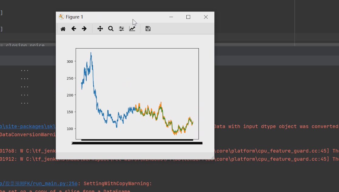
项目运行效果：

毕业设计 lstm股价预测

项目获取：

https://gitee.com/sinonfin/algorithm-sharing

1 LSTM 神经网络

长短期记忆 (LSTM) 神经网络属于循环神经网络 (RNN) 的一种，特别适合处理和预测与时间序列相关的重要事件。以下面的句子作为一个上下文推测的例子：

​
“我从小在法国长大，我会说一口流利的？？”

由于同一句话前面提到”法国“这个国家，且后面提到“说”这个动作。因此，LSTM便能从”法国“以及”说“这两个长短期记忆中重要的讯号推测出可能性较大的”法语“这个结果。

K线图与此类似，股价是随着时间的流动及重要讯号的出现而做出反应的：

• 在价稳量缩的盘整区间中突然出现一带量突破的大红K，表示股价可能要上涨了
• 在跳空缺口后出现岛状反转，表示股价可能要下跌了
• 在连涨几天的走势突然出现带有长上下影线的十字线，表示股价有反转的可能

LSTM 要做的事情就是找出一段时间区间的K棒当中有没有重要讯号（如带量红K）并学习预测之后股价的走势。

2 LSTM 股价预测实例

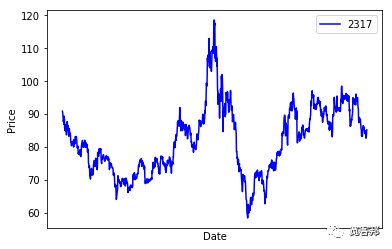
数据是以鸿海(2317)从2013年初到2017年底每天的开盘价、收盘价、最高价、最低价、以及成交量等数据。

首先将数据写入并存至pandas的DataFrame，另外对可能有N/A的row进行剔除：

数据写入：

​    
    import pandas as pd
    foxconndf= pd.read_csv('./foxconn_2013-2017.csv', index_col=0)
    foxconndf.dropna(how='any',inplace=True)

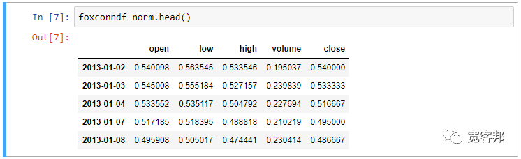
為了避免原始数据太大或是太小没有统一的范围而导致 LSTM 在训练时难以收敛，我们以一个最小最大零一正规化方法对数据进行修正：

​    
    from sklearn import preprocessing
    
   defnormalize(df):
        newdf= df.copy()
        min_max_scaler = preprocessing.MinMaxScaler()
        newdf['open']= min_max_scaler.fit_transform(df.open.values.reshape(-1,1))
        newdf['low']= min_max_scaler.fit_transform(df.low.values.reshape(-1,1))
        newdf['high']= min_max_scaler.fit_transform(df.high.values.reshape(-1,1))
        newdf['volume']= min_max_scaler.fit_transform(df.volume.values.reshape(-1,1))
        newdf['close']= min_max_scaler.fit_transform(df.close.values.reshape(-1,1))return newdf
    foxconndf_norm= normalize(foxconndf)

然后对数据进行训练集与测试集的切割，另外也定义每一笔数据要有多长的时间框架：

​

import numpy as np
def data_helper(df, time_frame):

3 数据维度: 开盘价、收盘价、最高价、最低价、成交量, 5维

number_features = len(df.columns)

# 将dataframe 转换为 numpy array
datavalue = df.as_matrix()

result = []
# 若想要观察的 time_frame 為20天, 需要多加一天作为验证答案
for index in range( len(datavalue) - (time_frame+1) ): # 从 datavalue 的第0个跑到倒数第 time_frame+1 个
    result.append(datavalue[index: index + (time_frame+1) ]) # 逐笔取出 time_frame+1 个K棒数值做為一笔 instance

result = np.array(result)
number_train = round(0.9 * result.shape[0]) # 取 result 的前90% instance 作为训练数据

x_train = result[:int(number_train), :-1] # 训练数据中, 只取每一个 time_frame 中除了最后一笔的所有数据作为feature
y_train = result[:int(number_train), -1][:,-1] # 训练数据中, 取每一个 time_frame 中最后一笔数据的最后一个数值(收盘价)作为答案

# 测试数据
x_test = result[int(number_train):, :-1]
y_test = result[int(number_train):, -1][:,-1]

# 将数据组成变好看一点
x_train = np.reshape(x_train, (x_train.shape[0], x_train.shape[1], number_features))
x_test = np.reshape(x_test, (x_test.shape[0], x_test.shape[1], number_features))  

return [x_train, y_train, x_test, y_test]

4 以20天为一区间进行股价预测

X_train, y_train, X_test, y_test = data_helper(foxconndf_norm,20)

我们以 Keras 框架作为 LSTM 的模型选择，首先在前面加了两层 256个神经元的 LSTM
layer，并都加上了Dropout层来防止数据过度拟合（overfitting）。最后再加上两层有不同数目神经元的全连结层来得到只有1维数值的输出结果，也就是预测股价：

​    
    from keras.models import Sequential
    from keras.layers.core import Dense, Dropout, Activation
    from keras.layers.recurrent import LSTM
    import keras
    
    defbuild_model(input_length, input_dim):
        d =0.3
        model = Sequential()
    
        model.add(LSTM(256, input_shape=(input_length, input_dim), return_sequences=True))
        model.add(Dropout(d))
    
        model.add(LSTM(256, input_shape=(input_length, input_dim), return_sequences=False))
        model.add(Dropout(d))
    
        model.add(Dense(16,kernel_initializer="uniform",activation='relu'))
        model.add(Dense(1,kernel_initializer="uniform",activation='linear'))
    
        model.compile(loss='mse',optimizer='adam', metrics=['accuracy'])return model
    
    # 20天、5维
    model = build_model(20,5)

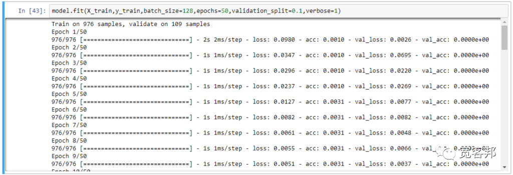
建立好 LSTM 模型后，我们就用前面编辑好的训练数据集开始进行模型的训练：LSTM 模型训练

​

# 一个batch有128个instance，总共跑50个迭代
    model.fit( X_train, y_train, batch_size=128, epochs=50, validation_split=0.1, verbose=1)

![dccbe8900b82f436d5a68d991f80179d.png](https://img-
blog.csdnimg.cn/img_convert/dccbe8900b82f436d5a68d991f80179d.png)

在经过一段时间的训练过程后，我们便能得到 LSTM
模型（model）。接着再用这个模型对测试数据进行预测，以及将预测出来的数值（pred）与实际股价（y_test）还原回原始股价的大小区间：

LSTM 模型预测股价及还原数值

​

defdenormalize(df, norm_value):
    original_value = df['close'].values.reshape(-1,1)
    norm_value = norm_value.reshape(-1,1)
    
    min_max_scaler = preprocessing.MinMaxScaler()
    min_max_scaler.fit_transform(original_value)
    denorm_value = min_max_scaler.inverse_transform(norm_value)return denorm_value

# 用训练好的 LSTM 模型对测试数据集进行预测
pred = model.predict(X_test)# 将预测值与实际股价还原回原来的区间值
denorm_pred = denormalize(foxconndf, pred)
denorm_ytest = denormalize(foxconndf, y_test)

5 LSTM 预测股价结果

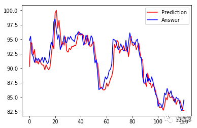
让我们把还原后的数值与实际股价画出来，看看效果如何：

LSTM 预测股价结果

​

import matplotlib.pyplot as plt
    %matplotlib inline  
    
    plt.plot(denorm_pred,color='red', label='Prediction')
    plt.plot(denorm_ytest,color='blue', label='Answer')
    plt.legend(loc='best')
    plt.show()

如下图，蓝线是实际股价、红线是预测股价。虽然整体看起来预测股价与实际股价有类似的走势，但仔细一看预测股价都比实际股价落后了几天。

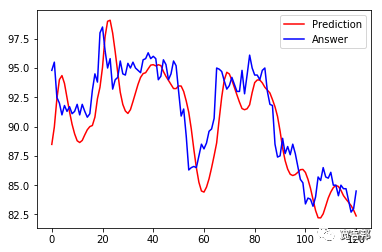
所以我们来调整一些设定：

• 时间框架长度的调整
• Keras 模型里全连结层的 activation 与 optimizaer 的调整
• Keras 模型用不同的神经网路（种类、顺序、数量）来组合batch_size 的调整、epochs 的调整 …

经过我们对上述的几个参数稍微调整过后，我们就得到一个更贴近实际股价的预测结果啦。

6 完整工程项目

项目分享：

https://gitee.com/sinonfin/algorithm-sharing