从零实现深度学习框架——手写前馈网络实现电影评论分类

引言

本着“凡我不能创造的，我就不能理解”的思想，本系列文章会基于纯Python以及NumPy从零创建自己的深度学习框架，该框架类似PyTorch能实现自动求导。

要深入理解深度学习，从零开始创建的经验非常重要，从自己可以理解的角度出发，尽量不使用外部完备的框架前提下，实现我们想要的模型。本系列文章的宗旨就是通过这样的过程，让大家切实掌握深度学习底层实现，而不是仅做一个调包侠。
本系列文章首发于微信公众号：JavaNLP

我们已经了解了前馈神经网络的基础知识，本文就基于前馈网络来解决实际问题——IMDB电影评论分类。

imdb数据集

imdb数据集是英文电影评论数据集，包含50000条两极分化的评论，数据集被分为25000条用于训练和25000条用于测试的评论。它们都包含50%的正面和50%的负面评论。

我们想要训练一个前馈网络能学到输入一段英文评论，判断这段评论是正面(表扬、鼓励)还是负面(狂喷)的，属于一个二分类问题。

我们先来看下数据集，为了简单，我们先用keras提供的封装方法加载数据集，需要引入

from keras.datasets import imdb

。

defload_dataset():# 保留训练数据中前10000个最常出现的单词，舍弃低频单词(X_train, y_train),(X_test, y_test)= imdb.load_data(num_words=10000)return Tensor(X_train), Tensor(X_test), Tensor(y_train), Tensor(y_test)defindices_to_sentence(indices: Tensor):# 单词索引字典 word -> index
    word_index = imdb.get_word_index()# 逆单词索引字典 index -> word
    reverse_word_index =dict([(value, key)for(key, value)in word_index.items()])# 将index列表转换为word列表## 0、1、2 是为“padding”（填充）、“start of sequence”（序# 列开始）、“unknown”（未知词）分别保留的索引
    decoded_review =' '.join([reverse_word_index.get(i -3,'?')for i in indices.data])return decoded_review

if __name__ =='__main__':
    X_train, X_test, y_train, y_test = load_dataset()print(indices_to_sentence(X_train[0]))print(y_train[0])

这里加载了第一个样本，将索引还原成句子，最后打印出该句子对应的标签。

? this film was just brilliant casting location scenery story direction everyone's really suited the part they played and you could just imagine being there robert ? is an amazing actor and now the same being director ? father came from the same scottish island as myself so i loved the fact there was a real connection with this film the witty remarks throughout the film were great it was just brilliant so much that i bought the film as soon as it was released for ? and would recommend it to everyone to watch and the fly fishing was amazing really cried at the end it was so sad and you know what they say if you cry at a film it must have been good and this definitely was also ? to the two little boy's that played the ? of norman and paul they were just brilliant children are often left out of the ? list i think because the stars that play them all grown up are such a big profile for the whole film but these children are amazing and should be praised for what they have done don't you think the whole story was so lovely because it was true and was someone's life after all that was shared with us all
Tensor(1.0, requires_grad=False) # 对应的类别

很长的一段评论，该评论被标记为正面(1)。

句子的处理

这是我们第一次接触NLP相关任务，虽然我们人类能很容易地看懂文字，但是让机器读懂文字不是一件容易的事。

这里用了最简单的方法，首先将句子拆分成一个个单词，然后构造一个词典来保存每个单词和其对应的序号(

imdb.get_word_index()

)，这里keras已经帮我们处理好了。

然后保存每个句子的时候，我们只需要保留句子中所有单词对应的序号列表即可，得到序号列表相当于将句子进行了数字化。只有数字化之后，计算机才能处理。

每个样本都是单词序列列表，因此我们需要将它们还原成句子，人类才能看得懂。

但是我们不能将整数序列直接输入神经网络。我们需要将列表转换为向量。我们这里对序列列表使用ont-hot编码。比如序列

[3,5]

会被转换为10000维的向量，只有索引3和5的元素是1，相当于标记了哪些单词出现在序列中，这是一个简单的句子向量化方法。

这里我们把每个句子转换成一个10000维的向量，这里的10000是我们设的最常见的单词数，包括填充词、序列开始词和未知词。每个句子都会有一个序列开始词，表示这是一个句子的开始单词；未知词是来处理不常见单词的，比如你不在这10000个常见单词里面的词；填充词用于填充句子；

defvectorize_sequences(sequences, dimension=10000):# 默认生成一个[句子长度，维度数]的向量
    results = np.zeros((len(sequences), dimension), dtype='uint8')for i, sequence inenumerate(sequences):# 将第i个序列中，对应单词序号处的位置置为1
        results[i, sequence]=1return results

X_train = vectorize_sequences(X_train)print(X_train[0])

[0 1 1 ... 0 0 0]

处理好句子之后，我们就可以将数据输入到神经网络中。

构建前馈神经网络

输入数据是向量，而标签是标量(1或0)，这和我们之前使用逻辑回归构建的模型一样，不过这次我们采用神经网络的方式。

我们使用前面介绍的单隐藏层前馈网络来处理这个问题，看一下效果如何。

首先设计我们的单隐藏层网络：

classFeedforward(nn.Module):'''
    简单单隐藏层前馈网络，用于分类问题
    '''def__init__(self, input_size, hidden_size, output_size):'''

        :param input_size: 输入维度
        :param hidden_size: 隐藏层大小
        :param output_size: 分类个数
        '''
        self.net = nn.Sequential(
            nn.Linear(input_size, hidden_size),# 隐藏层，将输入转换为隐藏向量
            nn.ReLU(),# 激活函数
            nn.Linear(hidden_size, output_size)# 输出层，将隐藏向量转换为输出)defforward(self, x: Tensor)-> Tensor:return self.net(x)

实现这种顺序网络很简单，就像堆叠石头一样，一层一层往上堆叠即可。

由于我们将使用之前介绍的BCELoss，因此最终的输出只是logits即可，不需要是经过Sigmoid的概率。

训练模型

由于我们的数据量足够大，我们可以从训练集中保留一部分数据作为验证集，以监控训练的效果。

# 保留验证集# X_train有25000条数据，我们保留10000条作为验证集
X_val = X_train[:10000]
X_train = X_train[10000:]

y_val = y_train[:10000]
y_train = y_train[10000:]

下面我们构造模型，并准备优化器和损失器，由于我们加了批处理，这里计算总损失，而不是均值。

model = Feedforward(10000,128,1)# 输入大小10000,隐藏层大小128，输出只有一个，代表判断为正例的概率

optimizer = SGD(model.parameters(), lr=0.001)# 先计算sum
loss = BCELoss(reduction="sum")

同时由于数据量较大，我们需要进行批处理，将训练集和验证集分成每批大小为512的批数据，训练20轮。

epochs =20
batch_size =512# 批大小
train_losses, val_losses =[],[]
train_accuracies, val_accuracies =[],[]# 由于数据过多，需要拆分成批次
X_train_batches, y_train_batches = make_batches(X_train, y_train,batch_size=batch_size)

X_val_batches, y_val_batches = make_batches(X_val, y_val, batch_size=batch_size)for epoch inrange(epochs):
    train_loss, train_accuracy = compute_loss_and_accury(X_train_batches, y_train_batches, model, loss,len(X_train), optimizer)

    train_losses.append(train_loss)
    train_accuracies.append(train_accuracy)with no_grad():
        val_loss, val_accuracy = compute_loss_and_accury(X_val_batches, y_val_batches, model, loss,len(X_val))

        val_losses.append(val_loss)
        val_accuracies.append(val_accuracy)print(f"Epoch:{epoch}, Train Loss: {train_loss:.4f}, Accuracy: {train_accuracy:.2f}% | "f" Validation Loss:{val_loss:.4f} , Accuracy:{val_accuracy:.2f}%")

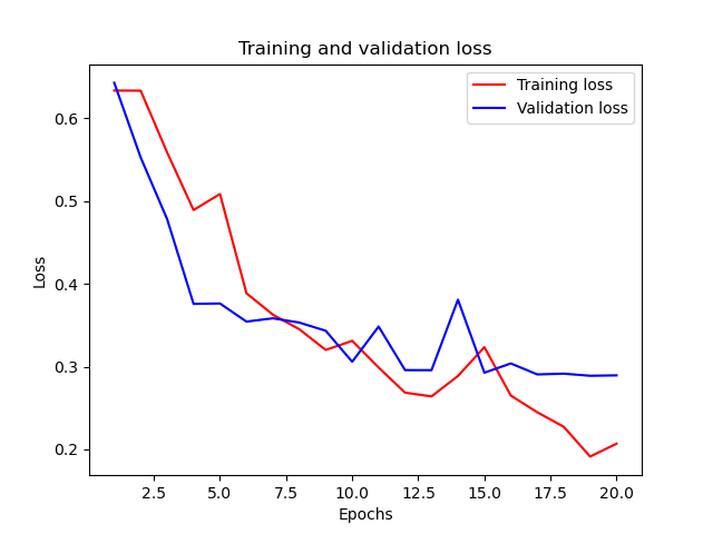
训练过程中的打印如下：

Epoch:1, Training Loss: 0.6335, Accuracy: 60.20% |  Validation Loss:0.6429 , Accuracy:49.55%
Epoch:2, Training Loss: 0.6333, Accuracy: 66.75% |  Validation Loss:0.5527 , Accuracy:76.28%
Epoch:3, Training Loss: 0.5587, Accuracy: 75.22% |  Validation Loss:0.4782 , Accuracy:82.10%
Epoch:4, Training Loss: 0.4891, Accuracy: 77.11% |  Validation Loss:0.3758 , Accuracy:84.26%
Epoch:5, Training Loss: 0.5085, Accuracy: 75.09% |  Validation Loss:0.3763 , Accuracy:83.28%
Epoch:6, Training Loss: 0.3887, Accuracy: 82.52% |  Validation Loss:0.3544 , Accuracy:84.76%
Epoch:7, Training Loss: 0.3628, Accuracy: 83.79% |  Validation Loss:0.3584 , Accuracy:85.17%
Epoch:8, Training Loss: 0.3451, Accuracy: 84.71% |  Validation Loss:0.3532 , Accuracy:83.87%
Epoch:9, Training Loss: 0.3201, Accuracy: 85.83% |  Validation Loss:0.3433 , Accuracy:84.42%
Epoch:10, Training Loss: 0.3311, Accuracy: 84.93% |  Validation Loss:0.3058 , Accuracy:87.20%
Epoch:11, Training Loss: 0.2989, Accuracy: 87.04% |  Validation Loss:0.3484 , Accuracy:83.60%
Epoch:12, Training Loss: 0.2685, Accuracy: 88.61% |  Validation Loss:0.2958 , Accuracy:87.65%
Epoch:13, Training Loss: 0.2640, Accuracy: 88.35% |  Validation Loss:0.2957 , Accuracy:87.72%
Epoch:14, Training Loss: 0.2887, Accuracy: 87.17% |  Validation Loss:0.3808 , Accuracy:82.40%
Epoch:15, Training Loss: 0.3235, Accuracy: 85.68% |  Validation Loss:0.2926 , Accuracy:87.75%
Epoch:16, Training Loss: 0.2650, Accuracy: 88.68% |  Validation Loss:0.3038 , Accuracy:86.86%
Epoch:17, Training Loss: 0.2448, Accuracy: 89.58% |  Validation Loss:0.2906 , Accuracy:87.94%
Epoch:18, Training Loss: 0.2273, Accuracy: 90.34% |  Validation Loss:0.2915 , Accuracy:88.05%
Epoch:19, Training Loss: 0.1913, Accuracy: 91.97% |  Validation Loss:0.2889 , Accuracy:88.33%
Epoch:20, Training Loss: 0.2069, Accuracy: 91.22% |  Validation Loss:0.2894 , Accuracy:88.07%

光看打印不够直观，我们可以绘制训练损失和验证损失：

还可以绘制训练和验证准确率的变化曲线：

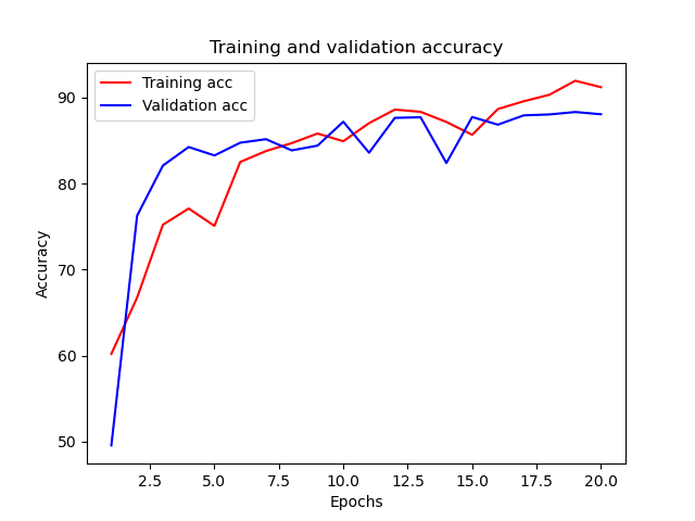
看起来模型还不错，但是真正怎么样还需要测试之后才知道，我们现在来预测没有看过的25000条记录：

# 最后在测试集上测试with no_grad():
   X_test, y_test = Tensor(X_test), Tensor(y_test)
   outputs = model(X_test)
   correct = np.sum(sigmoid(outputs).numpy().round()== y_test.numpy())
   accuracy =100* correct /len(y_test)print(f"Test Accuracy:{accuracy}")

Test Accuracy:88.004

嗯，我们直接纯手写实现的前馈网络模型和Keras的前馈模型表现差不多，还可以！

完整代码

完整代码笔者上传到了程序员最大交友网站上去了，地址: 👉 https://github.com/nlp-greyfoss/metagrad

References