
给定一个模型架构、数据类型、输入形状和优化器,你能否计算出前向传播和反向传播所需的GPU内存量?要回答这个问题,我们需要将流程分解为基本组件,并从底层理解内存需求。以下实验(可以在Google Colab上运行)将帮助你理解核心概念。
预留与分配
PyTorch预留了更多内存,但只分配所需的内存。这样做是为了在需要更多内存时能够快速分配,而不是进行昂贵的预留操作。我们只关心内存分配,而不关心预留。
 deftest_reservation_vs_allocation():
     print(f"Base memory reserved: {torch.cuda.memory_reserved(device_id)}")
     print(f"Base memory allocated: {torch.cuda.memory_allocated(device_id)}")

     # Allocate some memory
     x=torch.randn((1024,), dtype=torch.float32, device=device)
     print(f"Memory after allocation (reserved): {torch.cuda.memory_reserved(device_id)}")
     print(f"Memory after allocation (allocated): {torch.cuda.memory_allocated(device_id)}")

     # Cleanup
     delx
     print(f"Memory after cleanup (reserved): {torch.cuda.memory_reserved(device_id)}")
     print(f"Memory after cleanup (allocated): {torch.cuda.memory_allocated(device_id)}")

     torch.cuda.empty_cache()
     print(f"Memory after empty_cache (reserved): {torch.cuda.memory_reserved(device_id)}")
     print(f"Memory after empty_cache (allocated): {torch.cuda.memory_allocated(device_id)}")

 """
 Output:

 Base memory reserved: 0
 Base memory allocated: 0
 Memory after allocation (reserved): 2097152
 Memory after allocation (allocated): 4096
 Memory after cleanup (reserved): 2097152
 Memory after cleanup (allocated): 0
 Memory after empty_cache (reserved): 0
 Memory after empty_cache (allocated): 0
 """
当删除变量x或当x超出作用域时,x的内存被释放,但仍然为将来使用而预留。只有在调用
torch.cuda.empty_cache()
时,才会释放预留的内存。
这里的
torch.cuda.memory_allocated()
将返回PyTorch在此进程上分配的内存。如果有另一个进程正在使用一些GPU内存,将返回0。为了获取真实的GPU内存使用情况,可以使用以下函数。
 importsubprocess


 defget_gpu_memory_used(gpu_id):
     """
     Returns the amount of memory used on the specified GPU in bytes.

     Parameters:
     gpu_id (int): The ID of the GPU (e.g., 0 for "cuda:0", 1 for "cuda:1").

     Returns:
     int: The amount of memory used on the GPU in bytes.
     """
     try:
         # Run the nvidia-smi command to get memory usage
         result=subprocess.run(
             ["nvidia-smi", "--query-gpu=memory.used", "--format=csv,nounits,noheader", f"--id={gpu_id}"],
             stdout=subprocess.PIPE,
             text=True
         )

         # Get the used memory in MiB from the result
         used_memory_mib=int(result.stdout.strip())

         # Convert MiB to bytes (1 MiB = 1024 * 1024 bytes)
         used_memory_bytes=used_memory_mib*1024*1024

         returnused_memory_bytes

     exceptExceptionase:
         print(f"Error occurred: {e}")
         returnNone
数据类型
float32
需要4字节的内存,
bfloat16
需要2字节,我们可以绘制一些数据类型所需的内存图。
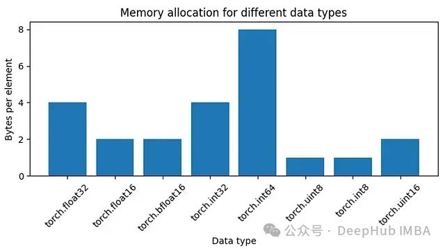
图1:不同数据类型的内存分配
 deftest_dtype_memory_allocation():
     dtypes= [torch.float32, torch.float16, torch.bfloat16, torch.int32, torch.int64, torch.uint8, torch.int8, torch.uint16]
     memories= []
     fordtypeindtypes:
         base_memory=get_gpu_memory_used(device_id)
         x=torch.ones((1024,), dtype=dtype, device=device)
         memory_after_allocation=get_gpu_memory_used(device_id)
         memories.append((memory_after_allocation-base_memory) //1024)
         delx
         torch.cuda.empty_cache()
     fig=plt.figure(figsize=(7, 4))
     fig.set_tight_layout(True)
     plt.bar([str(d) fordindtypes], memories)
     plt.xlabel("Data type")
     plt.ylabel("Bytes per element")
     plt.title("Memory allocation for different data types")
     plt.xticks(rotation=45)
     plt.show()
内存块
内存以512字节的块分配。当创建一个张量时,它被分配到下一个可用的块中。对于形状为(800,)的float32张量,不是分配800 * 4 = 3200字节,而是分配3584(512 * 7)字节。
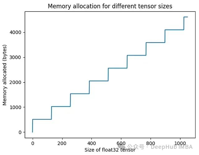
图2:不同张量大小的内存分配。
 deftest_memory_allocation_relationship():
     """
     For different sizes of tensors, check the memory allocated on GPU.
     """
     memories= []
     sizes=1050
     foriintqdm(range(sizes)):
         base_memory=get_gpu_memory_used(device_id)
         x=torch.randn((i,), dtype=torch.float32, device=device)
         memory_after_allocation=get_gpu_memory_used(device_id)
         memories.append(memory_after_allocation-base_memory)
         delx
         torch.cuda.empty_cache()
     plt.plot(memories)
     plt.xlabel("Size of float32 tensor")
     plt.ylabel("Memory allocated (bytes)")
     plt.title("Memory allocation for different tensor sizes")
     plt.show()
可训练参数(单个线性层前向传播)
接下来我们将看一个单一的线性层。进行前向传播,并计算所需的内存。
 deftest_single_linear_layer_forward_allocation():
     # Disable cublas
     # import os; os.environ["CUBLAS_WORKSPACE_CONFIG"] = ":0:0"

     print(f"Base memory: {torch.cuda.memory_allocated(device_id)}")

     model=nn.Linear(256, 250, device=device, dtype=torch.float32)
     print(f"Memory after model allocation: {torch.cuda.memory_allocated(device_id)}")

     x=torch.randn((1, 256,), dtype=torch.float32, device=device)
     print(f"Memory after input allocation: {torch.cuda.memory_allocated(device_id)}")

     y=model(x)
     final_memory=torch.cuda.memory_allocated(device_id)
     print(f"Memory after forward pass: {final_memory}")

     # Memory calculations
     w_mem=len(model.weight.flatten()) *model.weight.dtype.itemsize
     # Get the higher multiple of 512
     w_mem_as_chunks= (w_mem+511) //512*512
     print(f"{model.weight.shape=}, {w_mem=}, {w_mem_as_chunks=}")

     b_mem=len(model.bias) *model.bias.dtype.itemsize
     b_mem_as_chunks= (b_mem+511) //512*512
     print(f"{model.bias.shape=}, {b_mem=}, {b_mem_as_chunks=}")

     x_mem= (len(x.flatten()) *x.dtype.itemsize+511) //512*512
     y_mem= (len(y.flatten()) *y.dtype.itemsize+511) //512*512
     print(f"{x_mem=}, {y_mem=}")

     total_memory_expected=w_mem_as_chunks+b_mem_as_chunks+x_mem+y_mem

     cublas_workspace_size=8519680
     memory_with_cublas=total_memory_expected+cublas_workspace_size
     print(f"{total_memory_expected=}, {memory_with_cublas=}")

     assertfinal_memory==memory_with_cublas

     delmodel, x, y
     torch.cuda.empty_cache()
     print(f"Memory after cleanup: {torch.cuda.memory_allocated(device_id)}")

     torch._C._cuda_clearCublasWorkspaces()
     print(f"Memory after clearing cublas workspace: {torch.cuda.memory_allocated(device_id)}")

 """
 Output:
 Base memory: 0
 Memory after model allocation: 257024
 Memory after input allocation: 258048
 Memory after forward pass: 8778752
 model.weight.shape=torch.Size([250, 256]), w_mem=256000, w_mem_as_chunks=256000
 model.bias.shape=torch.Size([250]), b_mem=1000, b_mem_as_chunks=1024
 x_mem=1024, y_mem=1024
 total_memory_expected=259072, memory_with_cublas=8778752
 Memory after cleanup: 8519680
 Memory after clearing cublas workspace: 0
 """
model
有一个形状为(256, 250)的float32
weight
矩阵,占用(256 * 250 * 4) = 256,000字节,这正好是内存块大小512的倍数(512 * 500 = 256,000)。但是
bias
有250个float32需要占用(250 * 4) = 1000字节。而512的更高倍数是2,(512 * 2) = 1024字节。
x
和
y
是形状为(256,)的张量,所以它们各占用1024字节。总内存 =
weight
+
bias
+
x
+
y
当我们将所有内容加起来时,应该得到259,072字节(256,000 + 1024 + 1024 + 1024)。但是实际观察到的大小是8,778,752字节。这额外的8,519,680字节来自分配cuBLAS工作空间。
这是为快速矩阵乘法操作预留的内存空间。对于某些matmul操作,会分配一个新的8,519,680字节的块。这个大小可能会根据GPU和Python环境而变化。当调用
torch.cuda.empty_cache()
时,cublas内存不会消失。它需要
torch._C._cuda_clearCublasWorkspaces()
来实际清除它。也可以设置环境变量
os.environ["CUBLAS_WORKSPACE_CONFIG"] = ":0:0"
来禁用cublas工作空间。但这可能是一种以牺牲执行速度为代价来优化内存的方法,所以我们使用默认就好。
梯度(单个线性层反向传播)
使用相同的模型,运行
loss.backward()
。为简单起见假设损失为
loss = y.sum()
。
 deftest_single_linear_layer_backward_allocation():
     print(f"Base memory: {torch.cuda.memory_allocated(device_id)}")

     model=nn.Linear(256, 250, device=device, dtype=torch.float32)
     x=torch.randn((1, 256,), dtype=torch.float32, device=device)
     y=model(x)

     print(f"Memory after forward pass: {torch.cuda.memory_allocated(device_id)}")
     y.sum().backward()
     final_memory=torch.cuda.memory_allocated(device_id)
     print(f"Memory after backward pass: {final_memory}")

     # Memory calculations
     next_chunk=lambdan: (n+511) //512*512
     units=model.weight.dtype.itemsize  # 4 bytes for float32
     mem=next_chunk(len(model.weight.flatten()) *units)
     mem+=next_chunk(len(model.bias) *units)
     print(f"Excepted model memory: {mem}")

     x_mem=next_chunk(len(x.flatten()) *units)
     y_mem=next_chunk(len(y.flatten()) *units)
     print(f"{x_mem=}, {y_mem=}")
     mem+=x_mem+y_mem

     # Gradient memory
     w_grad_mem=next_chunk(len(model.weight.grad.flatten()) *units)
     b_grad_mem=next_chunk(len(model.bias.grad.flatten()) *units)
     print(f"{model.weight.grad.shape=}, {w_grad_mem=}")
     print(f"{model.bias.grad.shape=}, {b_grad_mem=}")
     mem+=w_grad_mem+b_grad_mem

     mem+=2*8519680  # cublas_size doubled
     print(f"Total memory expected: {mem}")
     assertfinal_memory==mem

     delmodel, x, y
     torch.cuda.empty_cache()
     print(f"Memory after cleanup: {torch.cuda.memory_allocated(device_id)}")

     torch._C._cuda_clearCublasWorkspaces()
     print(f"Memory after clearing cublas workspace: {torch.cuda.memory_allocated(device_id)}")

 """
 Output:
 Base memory: 0
 Memory after forward pass: 8778752
 Memory after backward pass: 17555456
 Excepted model memory: 257024
 x_mem=1024, y_mem=1024
 model.weight.grad.shape=torch.Size([250, 256]), w_grad_mem=256000
 model.bias.grad.shape=torch.Size([250]), b_grad_mem=1024
 Total memory expected: 17555456
 Memory after cleanup: 17039360
 Memory after clearing cublas workspace: 0
 """
由于每个具有
requires_grad=True
的模型参数都会有一个
.grad
成员来存储底层张量的梯度,所以模型的大小会翻倍。
这次分配了2个cublas工作空间内存块,假设一个用于前向传播,一个用于反向传播。此时cublas何时确切地分配新块还不确定。
中间张量(多层前馈网络)
当模型在推理模式下运行时,没有自动求导图,不需要存储中间张量。所以内存量只是简单地将每一层的内存相加。
在需要跟踪计算图的训练模式下情况会有所不同。当有多个串行应用的操作时,比如在前馈网络或任何深度网络中,自动求导图需要记住这些操作的中间张量。存储需求取决于它们的偏导数操作的性质。这些中间张量在反向传播过程中从内存中清除。我们看一些例子:
x
是输入,
w
是需要梯度的参数(
w.requires_grad = True
)。
x @ w不需要额外的存储。偏导数x已经存储。但是当x是某个输出,如x = u * w1时,x也需要被存储。x + w也不需要存储,因为对w的偏导数是0。(x * 2) @ w将需要存储操作数x * 2,因为它将用于找到梯度。(((x + 2) @ w1) + 3) * w2是一个有趣的案例,模仿了2层。 - 对于关于w1的偏导数,我们需要存储x + 2- 对于关于w2的偏导数,我们需要存储((x + 2) @ w1) + 3
让我们看看更深网络的实现:
 deftest_multi_layer_forward():
     print(f"Base memory: {torch.cuda.memory_allocated(device_id)}")

     inference_mode=False
     n_layers=1
     model=nn.Sequential(*[
         nn.Sequential(
             nn.Linear(200, 100),
             nn.ReLU(),  # No trainable params
             nn.Linear(100, 200),
             nn.Sigmoid(),  # No trainable params
         )
         for_inrange(n_layers)
     ]).to(device_id)
     batch_size=5
     x=torch.randn((batch_size, 200), device=device_id)
     withtorch.inference_mode(inference_mode):
         y=model(x)

     final_memory=torch.cuda.memory_allocated(device_id)
     print(f"Memory after forward pass: {final_memory}")

     # Computed memory
     next_chunk=lambdan: (n+511) //512*512
     mem=0
     unit=model[0][0].weight.dtype.itemsize
     forblockinmodel:
         forlayerinblock:
             ifisinstance(layer, nn.Linear):
                 mem+=next_chunk(len(layer.weight.flatten()) *unit)
                 mem+=next_chunk(len(layer.bias) *unit)
                 ifnotinference_mode:
                     # Gotta store the input
                     mem+=next_chunk(layer.in_features*batch_size*unit)
     mem+=next_chunk(len(y.flatten()) *unit)
     mem+=8519680  # cublas_size
     ifinference_mode:
         mem+=next_chunk(len(y.flatten()) *unit)
     print(f"Total memory expected: {mem}")
     assertfinal_memory==mem
在像BatchNorm1d、LayerNorm、RMSNorm这样的归一化层中,在与参数
w
相乘之前,有一个对输入
x
的操作,如
(x — x.mean()) / (x.std() + 1e-6) * w
。操作数
(x — x.mean()) / (x.std() + 1e-6)
是需要存储的中间输出。并且可能还有其他状态,如running_mean、running_std或
forward()
方法中的中间张量需要考虑。其中一些中间张量我们无法访问,所以我们无法确定发生了什么。当包含批量大小时,这变得更加复杂。
 deftest_layer_norm():
     print(f"Base memory: {torch.cuda.memory_allocated(device_id)}")
     x=torch.rand((10,), device=device_id)
     w=torch.rand((10,), requires_grad=True, device=device_id)
     # Layer Norm
     y= (x-x.mean()) / (x.std() +1e-6) *w
     final_memory=torch.cuda.memory_allocated(device_id)
     print(f"Memory after forward pass: {final_memory}")

     # Memory calculations
     next_chunk=lambdan: (n+511) //512*512
     mem=next_chunk(len(x.flatten()) *x.dtype.itemsize)
     mem+=next_chunk(len(w.flatten()) *w.dtype.itemsize)
     mem+=next_chunk(len(y.flatten()) *y.dtype.itemsize)
     mem+=next_chunk(len(x.flatten()) *x.dtype.itemsize)  # intermediate
     print(f"Total memory expected: {mem}")
     assertfinal_memory==mem
反向传播非常相似,但有一些变化:
- 模型大小因梯度存储而翻倍。
- 所有中间张量在最后都被清除。
- 分配了一个新的cublas工作空间。
 deftest_multi_layer_backward():
     print(f"Base memory: {torch.cuda.memory_allocated(device_id)}")

     n_layers=1
     model=nn.Sequential(*[
         nn.Sequential(
             nn.Linear(200, 100),
             nn.ReLU(),  # No trainable params
             nn.Linear(100, 200),
             nn.Sigmoid(),  # No trainable params
         )
         for_inrange(n_layers)
     ]).to(device_id)
     batch_size=5
     x=torch.randn((batch_size, 200), device=device_id)
     y=model(x)
     print(f"Memory after forward pass: {torch.cuda.memory_allocated(device_id)}")
     y.sum().backward()
     final_memory=torch.cuda.memory_allocated(device_id)
     print(f"Memory after backward pass: {final_memory}")

     # Computed memory
     next_chunk=lambdan: (n+511) //512*512
     mem=0
     unit=model[0][0].weight.dtype.itemsize
     forblockinmodel:
         forlayerinblock:
             ifisinstance(layer, nn.Linear):
                 mem+=next_chunk(len(layer.weight.flatten()) *unit) *2   # Weights and gradients
                 mem+=next_chunk(len(layer.bias) *unit) *2               # Biases and gradients
                 # mem += next_chunk(layer.in_features * batch_size * unit)  # Intermediate tensors are cleared
     mem+=next_chunk(len(y.flatten()) *unit)
     mem+=2*8519680                                                      # cublas_size doubled
     mem+=next_chunk(len(y.flatten()) *unit)
     print(f"Total memory expected: {mem}")
     assertfinal_memory==mem
优化器(单个线性层反向传播)
我们观察一些优化步骤的内存分配。
 deftest_single_linear_layer_with_optimizer():
     # Disable cublas
     importos; os.environ["CUBLAS_WORKSPACE_CONFIG"] =":0:0"

     memory_timeline_real= []
     add=lambdae: memory_timeline_real.append({"event": e, "memory": torch.cuda.memory_allocated(device_id)})
     add("baseline")

     in_size=256
     out_size=250
     batch_size=100
     model=nn.Linear(in_size, out_size, device=device, dtype=torch.float32)
     add("model_allocation")

     optimizer=torch.optim.Adam(model.parameters(), lr=0.001)
     add("optimizer_init")

     x=torch.randn((batch_size, in_size,), dtype=torch.float32, device=device)
     add("input_allocation")

     defstep(n):
         optimizer.zero_grad()
         add(f"optim_zero_grad_{n}")

         y=model(x)
         add(f"forward_{n}")

         y.sum().backward()
         add(f"backward_{n}")

         optimizer.step()
         dely
         add(f"optim_step_{n}")

     foriinrange(4):
         step(i+1)

     # Bar chart with even name on x-axis and total_memory on y-axis
     fig=plt.figure(figsize=(15, 7))
     fig.set_tight_layout(True)
     plt.ylim((0, 1_300_000))
     plt.bar([event["event"] foreventinmemory_timeline_real], [event["memory"] foreventinmemory_timeline_real])
     plt.xlabel("Event")
     plt.ylabel("Total memory allocated (bytes)")
     plt.title(f"Memory allocation during training ({type(optimizer)})")
     plt.xticks(rotation=45)
     plt.show()
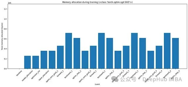
图3:使用SGD优化器在训练的各个阶段的内存分配
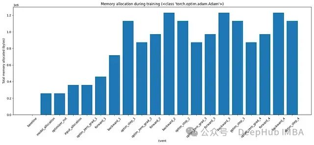
图4:使用Adam优化器在训练的各个阶段的内存分配
直到backward_1,我们看到内存分配如预期。当
optimizer.step()
结束时,在这个特定的代码中删除了
y
,所以该内存被释放。在底层优化器会获取额外的内存(等于可训练参数的大小)来更新它们,并在更新后释放该内存。这在图中没有显示。更详细的时间图可以在下图5中看到。
对于Adam对每个可训练参数都有一阶矩和二阶矩。所以它总是在内存中保留2倍的模型大小。这是这段代码中训练最耗费内存的部分。
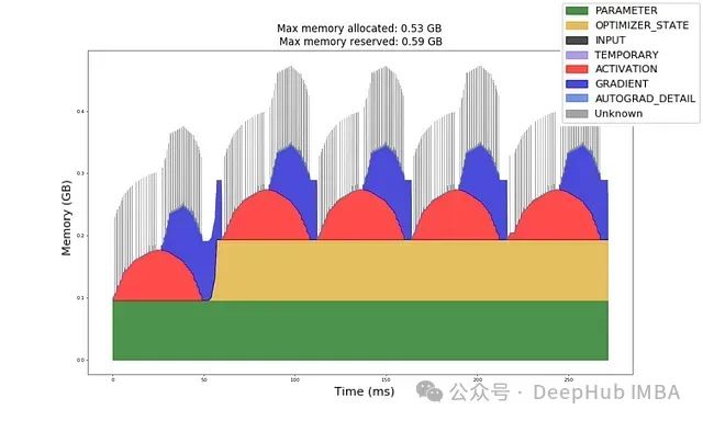
图5:按毫秒计的内存分配时间图。
现在让我们尝试手动计算这些内存需求:
 # Memory calculations (continuing from previous code block)
     units=model.weight.dtype.itemsize
     memory_timeline= []
     all_keys= ["trainable_params", "input", "output", "gradient", "intermediate_tensors", "optimizer_state"]
     defupdate_memory(event: str, update: dict):
         prev_state=memory_timeline[-1] ifmemory_timelineelse {k: 0forkinall_keys}
         new_state= {k: prev_state.get(k, 0) +update.get(k, 0) forkinall_keys}
         new_state["event"] =event
         memory_timeline.append(new_state)
     next_chunk=lambdan: (n+511) //512*512

     update_memory("baseline", {})

     # Model memory
     model_mem=next_chunk(len(model.weight.flatten()) *units)
     model_mem+=next_chunk(len(model.bias) *units)
     update_memory("model_allocation", {"trainable_params": model_mem})
     update_memory("optimizer_init", {})

     # Input memory
     x_mem=next_chunk(len(x.flatten()) *units)
     update_memory("input_allocation", {"input": x_mem})
     update_memory("optim_zero_grad_1", {})

     # Forward
     y_mem=next_chunk(batch_size*out_size*units)
     # Add any intermediate tensors here.
     update_memory("forward_1", {"output": y_mem})  # , "intermediate_tensors": ...})

     # Backward
     grad_mem=next_chunk(len(model.weight.grad.flatten()) *units)
     grad_mem+=next_chunk(len(model.bias.grad.flatten()) *units)
     # Clear any intermediate tensors here.
     update_memory("backward_1", {"gradient": grad_mem})  # "intermediate_tensors": ...})

     # Optimizer memory
     ifisinstance(optimizer, torch.optim.SGD):
         # SGD has parameters in memory. They are cleared after each step.
         optimizer_mem=0
     elifisinstance(optimizer, torch.optim.Adam):
         # Adam has parameters and 2 momentum buffers. Parameters are cleared after each step.
         optimizer_mem=2*model_mem
     else:
         raise
     update_memory("optim_step_1", {"optimizer_state": optimizer_mem, "output": -y_mem})

     forstepinrange(2, 5):
         update_memory(f"optim_zero_grad_{step}", {"gradient": -grad_mem})
         update_memory(f"forward_{step}", {"output": y_mem})
         update_memory(f"backward_{step}", {"gradient": grad_mem})
         update_memory(f"optim_step_{step}", {"output": -y_mem})

     # Make totals
     foreventinmemory_timeline:
         event["total"] =sum([vforvinevent.values() ifisinstance(v, int)])

     # Plot memory timeline
     importpandasaspd
     df=pd.DataFrame(memory_timeline, columns=all_keys+ ["event"])
     df.set_index("event", inplace=True, drop=True)
     df.plot(kind='bar', stacked=True, figsize=(15, 7), ylim=(0, 1_300_000), xlabel="Event", ylabel="Total memory allocated (bytes)", title=f"Memory allocation expected ({type(optimizer)})")
     plt.tight_layout()
     plt.xticks(rotation=45)
     plt.show()

     # Compare the two timelines
     fori, (real, expected) inenumerate(zip(memory_timeline_real, memory_timeline)):
         assertreal["memory"] ==expected["total"], f"Memory mismatch at {real['event']}: {real['memory']} != {expected['total']}"
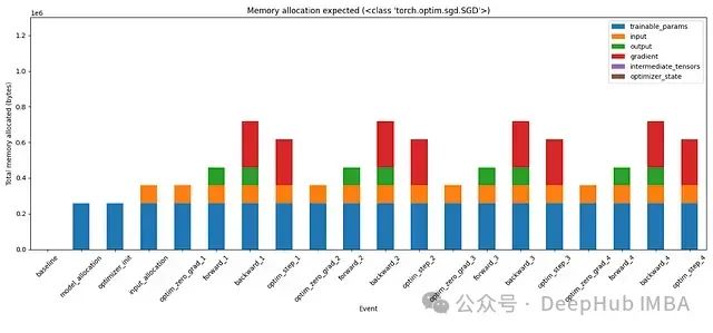
图6:使用SGD优化器在训练的不同阶段的内存使用分段
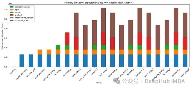
图7:使用Adam优化器在训练的不同阶段的内存使用分段
在手动计算内存分配后,我们的计算与观察结果相匹配。这次实际上可以看到内存分配到各种张量的分段。例如,Adam的状态占用了两倍的模型大小。梯度(红色)的不同变化。如果向继续测试,还可以尝试向这个模型添加更多层,添加中间张量并在适当的时候删除它们。这应该在这些条形图中创建另一个代表中间张量的分段。
总结
结合上面的每个概念我们可以回答主要问题:
- 可训练参数:固定的模型大小
- 内存块:它只以512字节的块出现
- Cublas内存:前向传播一个块,反向传播一个块
- 梯度:与模型大小相同
- 中间张量:最麻烦的部分,取决于代码如何编写
- 优化器:至少分配一倍的模型大小
最后一个问题就是,我们只处理了前馈层,那么CNN、Transformers、RNN等呢?首先CNN是类似前馈层的操作,所以我们可以根据他的计算规则进行计算,而Transformers、RNN都基础操作的组合,我们计算了一个前馈层可以根据他们的架构进行组合计算。我们已经掌握了计算前馈层内存需求的方法,所以我们可以自己解决这些问题!
作者:Akhilez