使用PyTorch复现ConvNext：从Resnet到ConvNext的完整步骤详解

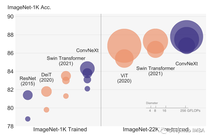
ConvNext论文提出了一种新的基于卷积的架构，不仅超越了基于 Transformer 的模型（如 Swin），而且可以随着数据量的增加而扩展！今天我们使用Pytorch来对其进行复现。下图显示了针对不同数据集/模型大小的 ConvNext 准确度。

作者首先采用众所周知的 ResNet 架构，并根据过去十年中的新最佳实践和发现对其进行迭代改进。作者专注于 Swin-Transformer，并密切关注其设计。这篇论文我们在以前也推荐过，如果你们有阅读过，我们强烈推荐阅读它:)

下图显示了所有各种改进以及每一项改进之后的各自性能。

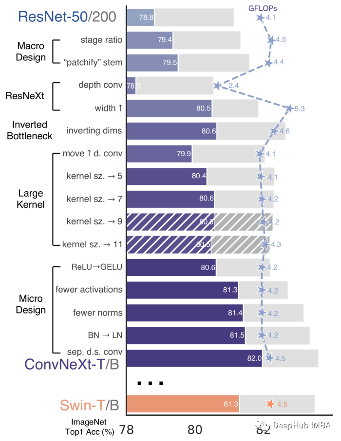
论文将设计的路线图分为两部分：宏观设计和微观设计。宏观设计是从高层次的角度所做的所有改变，例如架构的设计，而微设计更多的是关于细节的，例如激活函数，归一化等。

下面我们将从一个经典的 BottleNeck 块开始，并使用pytorch逐个实现论文中说到的每个更改。

从ResNet开始

ResNet 由一个一个的残差（BottleNeck）块，我们就从这里开始。

fromtorchimportnn
fromtorchimportTensor
fromtypingimportList
classConvNormAct(nn.Sequential):
    """
    A little util layer composed by (conv) -> (norm) -> (act) layers.
    """
    def__init__(
        self,
        in_features: int,
        out_features: int,
        kernel_size: int,
        norm = nn.BatchNorm2d,
        act = nn.ReLU,
        **kwargs
    ):
        super().__init__(
            nn.Conv2d(
                in_features,
                out_features,
                kernel_size=kernel_size,
                padding=kernel_size//2,
                **kwargs
            ),
            norm(out_features),
            act(),
        )
classBottleNeckBlock(nn.Module):
    def__init__(
        self,
        in_features: int,
        out_features: int,
        reduction: int = 4,
        stride: int = 1,
    ):
        super().__init__()
        reduced_features = out_features//reduction
        self.block = nn.Sequential(
            # wide -> narrow
            ConvNormAct(
                in_features, reduced_features, kernel_size=1, stride=stride, bias=False
            ),
            # narrow -> narrow
            ConvNormAct(reduced_features, reduced_features, kernel_size=3, bias=False),
            # narrow -> wide
            ConvNormAct(reduced_features, out_features, kernel_size=1, bias=False, act=nn.Identity),
        )
        self.shortcut = (
            nn.Sequential(
                ConvNormAct(
                    in_features, out_features, kernel_size=1, stride=stride, bias=False
                )
            )
            ifin_features!= out_features
            elsenn.Identity()
        )
        self.act = nn.ReLU()
    defforward(self, x: Tensor) ->Tensor:
        res = x
        x = self.block(x)
        res = self.shortcut(res)
        x += res
        x = self.act(x)
        returnx

看看上面代码是否有效

importtorch
x = torch.rand(1, 32, 7, 7)
block = BottleNeckBlock(32, 64)
block(x).shape
#torch.Size([1, 64, 7, 7])

下面开始定义Stage，Stage也叫阶段是残差块的集合。每个阶段通常将输入下采样 2 倍

classConvNexStage(nn.Sequential):
    def__init__(
        self, in_features: int, out_features: int, depth: int, stride: int = 2, **kwargs
    ):
        super().__init__(
            # downsample is done here
            BottleNeckBlock(in_features, out_features, stride=stride, **kwargs),
            *[
                BottleNeckBlock(out_features, out_features, **kwargs)
                for_inrange(depth-1)
            ],
        )

测试

stage = ConvNexStage(32, 64, depth=2)
stage(x).shape
#torch.Size([1, 64, 4, 4])

我们已经将输入是从 7x7 减少到 4x4 。

ResNet 也有所谓的 stem，这是模型中对输入图像进行大量下采样的第一层。

classConvNextStem(nn.Sequential):
    def__init__(self, in_features: int, out_features: int):
        super().__init__(
            ConvNormAct(
                in_features, out_features, kernel_size=7, stride=2
            ),
            nn.MaxPool2d(kernel_size=3, stride=2, padding=1),
        )

现在我们可以定义 ConvNextEncoder 来拼接各个阶段，并将图像作为输入生成最终嵌入。

classConvNextEncoder(nn.Module):
    def__init__(
        self,
        in_channels: int,
        stem_features: int,
        depths: List[int],
        widths: List[int],
    ):
        super().__init__()
        self.stem = ConvNextStem(in_channels, stem_features)
        in_out_widths = list(zip(widths, widths[1:]))
        self.stages = nn.ModuleList(
            [
                ConvNexStage(stem_features, widths[0], depths[0], stride=1),
                *[
                    ConvNexStage(in_features, out_features, depth)
                    for (in_features, out_features), depthinzip(
                        in_out_widths, depths[1:]
                    )
                ],
            ]
        )
    defforward(self, x):
        x = self.stem(x)
        forstageinself.stages:
            x = stage(x)
        returnx

测试结果如下：

image = torch.rand(1, 3, 224, 224)
encoder = ConvNextEncoder(in_channels=3, stem_features=64, depths=[3,4,6,4], widths=[256, 512, 1024, 2048])
encoder(image).shape
#torch.Size([1, 2048, 7, 7])

现在我们完成了 resnet50 编码器，如果你附加一个分类头，那么他就可以在图像分类任务上工作。下面开始进入本文的正题实现ConvNext。

Macro Design

1、改变阶段计算比率

传统的ResNet 中包含了 4 个阶段，而Swin Transformer这4个阶段使用的比例为1:1:3:1(第一个阶段有一个区块，第二个阶段有一个区块，第三个阶段有三个区块……)将ResNet50调整为这个比率((3,4,6,3)->(3,3,9,3))可以使性能从78.8%提高到79.4%。

encoder = ConvNextEncoder(in_channels=3, stem_features=64, depths=[3,3,9,3], widths=[256, 512, 1024, 2048])

2、将stem改为“Patchify”

ResNet stem使用的是非常激进的7x7和maxpool来大量采样输入图像。然而，Transfomers 使用了被称为“Patchify”的主干，这意味着他们将输入图像嵌入到补丁中。Vision transforms使用非常激进的补丁(16x16)，而ConvNext的作者使用使用conv层实现的4x4补丁，这使得性能从79.4%提升到79.5%。

classConvNextStem(nn.Sequential):
    def__init__(self, in_features: int, out_features: int):
        super().__init__(
            nn.Conv2d(in_features, out_features, kernel_size=4, stride=4),
            nn.BatchNorm2d(out_features)
        )

3、ResNeXtify

ResNetXt 对 BottleNeck 中的 3x3 卷积层采用分组卷积来减少 FLOPS。在 ConvNext 中使用depth-wise convolution（如 MobileNet 和后来的 EfficientNet）。depth-wise convolution也是是分组卷积的一种形式，其中组数等于输入通道数。

作者注意到这与 self-attention 中的加权求和操作非常相似，后者仅在空间维度上混合信息。使用 depth-wise convs 会降低精度（因为没有像 ResNetXt 那样增加宽度），这是意料之中的毕竟提升了速度。

所以我们将 BottleNeck 块内的 3x3 conv 更改为下面代码

ConvNormAct(reduced_features, reduced_features, kernel_size=3, bias=False, groups=reduced_features)

4、Inverted Bottleneck（倒置瓶颈）

一般的 BottleNeck 首先通过 1x1 conv 减少特征，然后用 3x3 conv，最后将特征扩展为原始大小，而倒置瓶颈块则相反。

所以下面我们从宽 -> 窄 -> 宽修改到到窄 -> 宽 -> 窄。

这与 Transformer 类似，由于 MLP 层遵循窄 -> 宽 -> 窄设计，MLP 中的第二个稠密层将输入的特征扩展了四倍。

classBottleNeckBlock(nn.Module):
    def__init__(
        self,
        in_features: int,
        out_features: int,
        expansion: int = 4,
        stride: int = 1,
    ):
        super().__init__()
        expanded_features = out_features*expansion
        self.block = nn.Sequential(
            # narrow -> wide
            ConvNormAct(
                in_features, expanded_features, kernel_size=1, stride=stride, bias=False
            ),
            # wide -> wide (with depth-wise)
            ConvNormAct(expanded_features, expanded_features, kernel_size=3, bias=False, groups=in_features),
            # wide -> narrow
            ConvNormAct(expanded_features, out_features, kernel_size=1, bias=False, act=nn.Identity),
        )
        self.shortcut = (
            nn.Sequential(
                ConvNormAct(
                    in_features, out_features, kernel_size=1, stride=stride, bias=False
                )
            )
            ifin_features!= out_features
            elsenn.Identity()
        )
        self.act = nn.ReLU()
    defforward(self, x: Tensor) ->Tensor:
        res = x
        x = self.block(x)
        res = self.shortcut(res)
        x += res
        x = self.act(x)
        returnx

5、扩大卷积核大小

像Swin一样，ViT使用更大的内核尺寸(7x7)。增加内核的大小会使计算量更大，所以才使用上面提到的depth-wise convolution，通过使用更少的通道来减少计算量。作者指出，这类似于 Transformers 模型，其中多头自我注意 (MSA) 在 MLP 层之前完成。

classBottleNeckBlock(nn.Module):
    def__init__(
        self,
        in_features: int,
        out_features: int,
        expansion: int = 4,
        stride: int = 1,
    ):
        super().__init__()
        expanded_features = out_features*expansion
        self.block = nn.Sequential(
            # narrow -> wide (with depth-wise and bigger kernel)
            ConvNormAct(
                in_features, in_features, kernel_size=7, stride=stride, bias=False, groups=in_features
            ),
            # wide -> wide 
            ConvNormAct(in_features, expanded_features, kernel_size=1),
            # wide -> narrow
            ConvNormAct(expanded_features, out_features, kernel_size=1, bias=False, act=nn.Identity),
        )
        self.shortcut = (
            nn.Sequential(
                ConvNormAct(
                    in_features, out_features, kernel_size=1, stride=stride, bias=False
                )
            )
            ifin_features!= out_features
            elsenn.Identity()
        )
        self.act = nn.ReLU()
    defforward(self, x: Tensor) ->Tensor:
        res = x
        x = self.block(x)
        res = self.shortcut(res)
        x += res
        x = self.act(x)
        returnx

这将准确度从 79.9% 提高到 80.6%

Micro Design

1、用 GELU 替换 ReLU

transformers使用的是GELU，为什么我们不用呢？作者测试替换后准确率保持不变。PyTorch 的GELU 是在 nn.GELU。

2、更少的激活函数

残差块有三个激活函数。而在Transformer块中，只有一个激活函数，即MLP块中的激活函数。作者除去了除中间层之后的所有激活。这是与swing - t一样的，这使得精度提高到81.3% !

3、更少的归一化层

与激活类似，Transformers 块具有较少的归一化层。作者决定删除所有 BatchNorm，只保留中间转换之前的那个。

4、用 LN 代替 BN

作者用 LN代替了 BN层。他们注意到在原始 ResNet 中提到这样做会损害性能，但经过作者以上的所有的更改后，性能提高到 81.5%

上面4个步骤让我们整合起来操作：

classBottleNeckBlock(nn.Module):
    def__init__(
        self,
        in_features: int,
        out_features: int,
        expansion: int = 4,
        stride: int = 1,
    ):
        super().__init__()
        expanded_features = out_features*expansion
        self.block = nn.Sequential(
            # narrow -> wide (with depth-wise and bigger kernel)
            nn.Conv2d(
                in_features, in_features, kernel_size=7, stride=stride, bias=False, groups=in_features
            ),
            # GroupNorm with num_groups=1 is the same as LayerNorm but works for 2D data
            nn.GroupNorm(num_groups=1, num_channels=in_features),
            # wide -> wide 
            nn.Conv2d(in_features, expanded_features, kernel_size=1),
            nn.GELU(),
            # wide -> narrow
            nn.Conv2d(expanded_features, out_features, kernel_size=1),
        )
        self.shortcut = (
            nn.Sequential(
                ConvNormAct(
                    in_features, out_features, kernel_size=1, stride=stride, bias=False
                )
            )
            ifin_features!= out_features
            elsenn.Identity()
        )
    defforward(self, x: Tensor) ->Tensor:
        res = x
        x = self.block(x)
        res = self.shortcut(res)
        x += res
        returnx

分离下采样层

在 ResNet 中，下采样是通过 stride=2 conv 完成的。Transformers（以及其他卷积网络）也有一个单独的下采样模块。作者删除了 stride=2 并在三个 conv 之前添加了一个下采样块，为了保持训练期间的稳定性在，在下采样操作之前需要进行归一化。将此模块添加到 ConvNexStage。达到了超过 Swin 的 82.0%！

classConvNexStage(nn.Sequential):
    def__init__(
        self, in_features: int, out_features: int, depth: int, **kwargs
    ):
        super().__init__(
            # add the downsampler
            nn.Sequential(
                nn.GroupNorm(num_groups=1, num_channels=in_features),
                nn.Conv2d(in_features, out_features, kernel_size=2, stride=2)
            ),
            *[
                BottleNeckBlock(out_features, out_features, **kwargs)
                for_inrange(depth)
            ],
        )

现在我们得到了最终的 BottleNeckBlock层代码：

classBottleNeckBlock(nn.Module):
    def__init__(
        self,
        in_features: int,
        out_features: int,
        expansion: int = 4,
    ):
        super().__init__()
        expanded_features = out_features*expansion
        self.block = nn.Sequential(
            # narrow -> wide (with depth-wise and bigger kernel)
            nn.Conv2d(
                in_features, in_features, kernel_size=7, padding=3, bias=False, groups=in_features
            ),
            # GroupNorm with num_groups=1 is the same as LayerNorm but works for 2D data
            nn.GroupNorm(num_groups=1, num_channels=in_features),
            # wide -> wide 
            nn.Conv2d(in_features, expanded_features, kernel_size=1),
            nn.GELU(),
            # wide -> narrow
            nn.Conv2d(expanded_features, out_features, kernel_size=1),
        )
    defforward(self, x: Tensor) ->Tensor:
        res = x
        x = self.block(x)
        x += res
        returnx

让我们测试一下最终的stage代码

stage = ConvNexStage(32, 62, depth=1)
stage(torch.randn(1, 32, 14, 14)).shape
#torch.Size([1, 62, 7, 7])

最后的一些丢该

论文中还添加了Stochastic Depth，也称为 Drop Path还有 Layer Scale。

fromtorchvision.opsimportStochasticDepth
classLayerScaler(nn.Module):
    def__init__(self, init_value: float, dimensions: int):
        super().__init__()
        self.gamma = nn.Parameter(init_value*torch.ones((dimensions)), 
                                    requires_grad=True)
        
    defforward(self, x):
        returnself.gamma[None,...,None,None] *x
classBottleNeckBlock(nn.Module):
    def__init__(
        self,
        in_features: int,
        out_features: int,
        expansion: int = 4,
        drop_p: float = .0,
        layer_scaler_init_value: float = 1e-6,
    ):
        super().__init__()
        expanded_features = out_features*expansion
        self.block = nn.Sequential(
            # narrow -> wide (with depth-wise and bigger kernel)
            nn.Conv2d(
                in_features, in_features, kernel_size=7, padding=3, bias=False, groups=in_features
            ),
            # GroupNorm with num_groups=1 is the same as LayerNorm but works for 2D data
            nn.GroupNorm(num_groups=1, num_channels=in_features),
            # wide -> wide 
            nn.Conv2d(in_features, expanded_features, kernel_size=1),
            nn.GELU(),
            # wide -> narrow
            nn.Conv2d(expanded_features, out_features, kernel_size=1),
        )
        self.layer_scaler = LayerScaler(layer_scaler_init_value, out_features)
        self.drop_path = StochasticDepth(drop_p, mode="batch")
        
    defforward(self, x: Tensor) ->Tensor:
        res = x
        x = self.block(x)
        x = self.layer_scaler(x)
        x = self.drop_path(x)
        x += res
        returnx

好了，现在我们看看最终结果

stage = ConvNexStage(32, 62, depth=1)
stage(torch.randn(1, 32, 14, 14)).shape
#torch.Size([1, 62, 7, 7])

最后我们修改一下Drop Path的概率

classConvNextEncoder(nn.Module):
    def__init__(
        self,
        in_channels: int,
        stem_features: int,
        depths: List[int],
        widths: List[int],
        drop_p: float = .0,
    ):
        super().__init__()
        self.stem = ConvNextStem(in_channels, stem_features)
        in_out_widths = list(zip(widths, widths[1:]))
        # create drop paths probabilities (one for each stage)
        drop_probs = [x.item() forxintorch.linspace(0, drop_p, sum(depths))] 
        
        self.stages = nn.ModuleList(
            [
                ConvNexStage(stem_features, widths[0], depths[0], drop_p=drop_probs[0]),
                *[
                    ConvNexStage(in_features, out_features, depth, drop_p=drop_p)
                    for (in_features, out_features), depth, drop_pinzip(
                        in_out_widths, depths[1:], drop_probs[1:]
                    )
                ],
            ]
        )
        
    defforward(self, x):
        x = self.stem(x)
        forstageinself.stages:
            x = stage(x)
        returnx

测试：

image = torch.rand(1, 3, 224, 224)
encoder = ConvNextEncoder(in_channels=3, stem_features=64, depths=[3,4,6,4], widths=[256, 512, 1024, 2048])
encoder(image).shape
#torch.Size([1, 2048, 3, 3])

ConvNext的特征，我们需要在编码器顶部应用分类头。我们还在最后一个线性层之前添加了一个 LayerNorm。

classClassificationHead(nn.Sequential):
    def__init__(self, num_channels: int, num_classes: int = 1000):
        super().__init__(
            nn.AdaptiveAvgPool2d((1, 1)),
            nn.Flatten(1),
            nn.LayerNorm(num_channels),
            nn.Linear(num_channels, num_classes)
        )
    
    
classConvNextForImageClassification(nn.Sequential):
    def__init__(self,  
                 in_channels: int,
                 stem_features: int,
                 depths: List[int],
                 widths: List[int],
                 drop_p: float = .0,
                 num_classes: int = 1000):
        super().__init__()
        self.encoder = ConvNextEncoder(in_channels, stem_features, depths, widths, drop_p)
        self.head = ClassificationHead(widths[-1], num_classes)

最终模型测试：

image = torch.rand(1, 3, 224, 224)
classifier = ConvNextForImageClassification(in_channels=3, stem_features=64, depths=[3,4,6,4], widths=[256, 512, 1024, 2048])
classifier(image).shape
#torch.Size([1, 1000])

最后总结

在本文中复现了作者使用ResNet 创建ConvNext 的所有过程。如果你想需要完整代码，可以查看这个地址：https://github.com/FrancescoSaverioZuppichini/ConvNext

这个地址是论文提供的官方代码，也可以参考：https://github.com/facebookresearch/ConvNeXt

作者：Francesco Zuppichini

标签：神经网络深度学习计算机视觉

使用PyTorch复现ConvNext：从Resnet到ConvNext的完整步骤详解

从ResNet开始

Macro Design

Micro Design

分离下采样层

最后的一些丢该

最后总结

发表评论

“使用PyTorch复现ConvNext：从Resnet到ConvNext的完整步骤详解”的评论:

关于作者

Deephub

相关阅读

文章导航