
介绍
决策树是一种用于监督学习的算法。它使用树结构,其中包含两种类型的节点:决策节点和叶节点。决策节点通过在要素上询问布尔值将数据分为两个分支。叶节点代表一个类。训练过程是关于在具有特定特征的特定特征中找到“最佳”分割。预测过程是通过沿着路径的每个决策节点回答问题来从根到达叶节点。
基尼不纯度和熵
术语“最佳”拆分是指拆分之后,两个分支比任何其他可能的拆分更“有序”。我们如何定义更多有序的?这取决于我们选择哪种指标。通常,度量有两种类型:基尼不纯度和熵。这些指标越小,数据集就越“有序”。
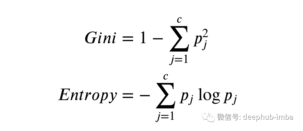
这两个指标之间的差异非常微妙。但 在大多数应用中,两个指标的行为类似。以下是用于计算每个指标的代码。
def gini_impurity(y):
    # calculate gini_impurity given labels/classes of each example
    m = y.shape[0]
    cnts = dict(zip(*np.unique(y, return_counts = True)))
    impurity = 1 - sum((cnt/m)**2 for cnt in cnts.values())
    return impurity

def entropy(y):
    # calculate entropy given labels/classes of each example
    m = y.shape[0]
    cnts = dict(zip(*np.unique(y, return_counts = True)))
    disorder = - sum((cnt/m)*log(cnt/m) for cnt in cnts.values())
    return disorder
构建树
训练过程实质上是在树上建树。关键步骤是确定“最佳”分配。过程如下:我们尝试按每个功能中的每个唯一值分割数据,然后选择混乱程度最小的最佳数据。现在我们可以将此过程转换为python代码。
def get_split(X, y):
    # loop through features and values to find best combination with the most information gain
    best_gain, best_index, best_value = 0, None, None
    cur_gini = gini_impurity(y)
    n_features = X.shape[1]

    for index in range(n_features):
        values = np.unique(X[:, index], return_counts = False)

        for value in values:
            left, right = test_split(index, value, X, y)
            if left['y'].shape[0] == 0 or right['y'].shape[0] == 0:
                continue
            gain = info_gain(left['y'], right['y'], cur_gini)
            if gain > best_gain:
                best_gain, best_index, best_value = gain, index, value
    best_split = {'gain': best_gain, 'index': best_index, 'value': best_value}
    return best_split

def test_split(index, value, X, y):
    # split a group of examples based on given index (feature) and value
    mask = X[:, index] < value
    left = {'X': X[mask, :], 'y': y[mask]}
    right = {'X': X[~mask, :], 'y': y[~mask]}
    return left, right

def info_gain(l_y, r_y, cur_gini):
    # calculate the information gain for a certain split
    m, n = l_y.shape[0], r_y.shape[0]
    p = m / (m + n)
    return cur_gini - p * gini_impurity(l_y) - (1 - p) * gini_impurity(r_y)
在构建树之前,我们先定义决策节点和叶节点。决策节点指定将在其上拆分的特征和值。它还指向左,右子项。叶节点包括类似于Counter对象的字典,该字典显示每个类有多少训练示例。这对于计算训练的准确性很有用。另外,它导致到达该叶子的每个示例的结果预测。
class Decision_Node:
    # define a decision node
    def __init__(self, index, value, left, right):
        self.index, self.value = index, value
        self.left, self.right = left, right

class Leaf:
    # define a leaf node
    def __init__(self, y):
        self.counts = dict(zip(*np.unique(y, return_counts = True)))
        self.prediction = max(self.counts.keys(), key = lambda x: self.counts[x])
鉴于其结构,通过递归构造树是最方便的。递归的出口是叶节点。当我们无法通过拆分提高数据纯度时,就会发生这种情况。如果我们可以找到“最佳”拆分,则这将成为决策节点。然后,我们对其左,右子级递归执行相同的操作。
def decision_tree(X, y):
    # train the decision tree model with a dataset
    correct_prediction = 0

    def build_tree(X, y):
        # recursively build the tree
        split = get_split(X, y)

        if split['gain'] == 0:
            nonlocal correct_prediction
            leaf = Leaf(y)
            correct_prediction += leaf.counts[leaf.prediction]
            return leaf

        left, right = test_split(split['index'], split['value'], X, y)
        left_node = build_tree(left['X'], left['y'])
        right_node = build_tree(right['X'], right['y'])

        return Decision_Node(split['index'], split['value'], left_node, right_node)

    root = build_tree(X, y)
    return correct_prediction/y.shape[0], root
预测
现在我们可以遍历树直到叶节点来预测一个示例。
def predict(x, node):
    if isinstance(node, Leaf):
        return node.prediction

    if x[node.index] < node.value:
        return predict(x, node.left)
    else:
        return predict(x, node.right)
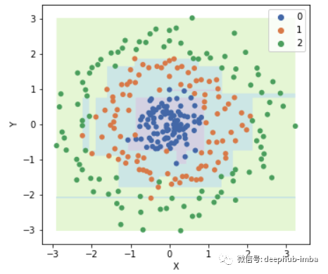
事实证明,训练精度为100%,决策边界看起来很奇怪!显然,该模型过度拟合了训练数据。好吧,如果考虑到这一点,如果我们继续拆分直到数据集变得更纯净,决策树将过度适合数据。换句话说,如果我们不停止分裂,该模型将正确分类每个示例!训练准确性为100%(除非具有完全相同功能的不同类别的示例),这丝毫不令人惊讶。
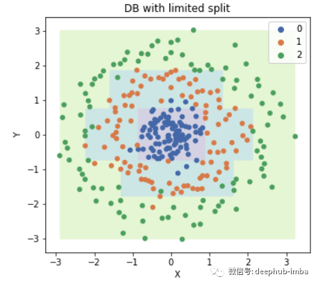
如何应对过度拟合?
从上一节中,我们知道决策树过拟合的幕后原因。为了防止过度拟合,我们需要在某个时候停止拆分树。因此,我们需要引入两个用于训练的超参数。它们是:树的最大深度和叶子的最小尺寸。让我们重写树的构建部分。
def decision_tree(X, y, max_dep = 5, min_size = 10):
    # train the decision tree model with a dataset
    correct_prediction = 0

    def build_tree(X, y, dep, max_dep = max_dep, min_size = min_size):
        # recursively build the tree
        split = get_split(X, y)

        if split['gain'] == 0 or dep >= max_dep or y.shape[0] <= min_size:
            nonlocal correct_prediction
            leaf = Leaf(y)
            correct_prediction += leaf.counts[leaf.prediction]
            return leaf

        left, right = test_split(split['index'], split['value'], X, y)

        left_node = build_tree(left['X'], left['y'], dep + 1)
        right_node = build_tree(right['X'], right['y'], dep + 1)

        return Decision_Node(split['index'], split['value'], left_node, right_node)

    root = build_tree(X, y, 0)

    return correct_prediction/y.shape[0], root
现在我们可以重新训练数据并绘制决策边界。
树的可视化
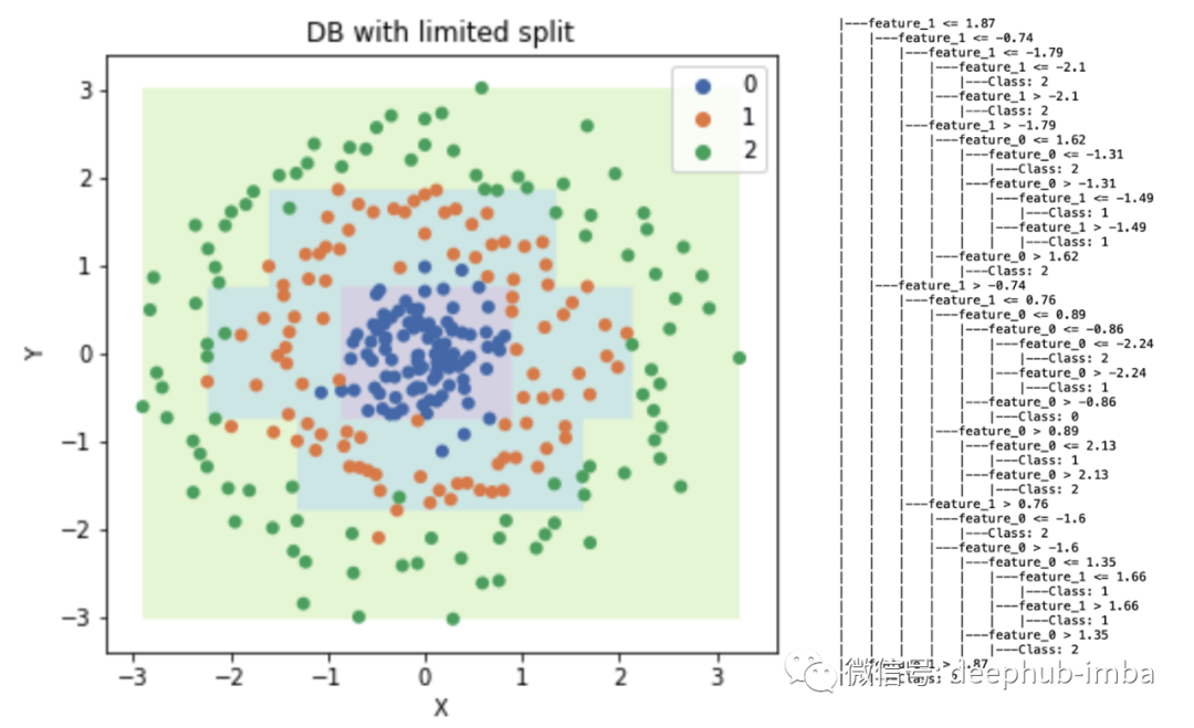
接下来,我们将通过打印出决策树的节点来可视化决策树。节点的压痕与其深度成正比。
def print_tree(node, indent = "|---"):
    # print the tree
    if isinstance(node, Leaf):
        print(indent + 'Class:', node.prediction)
        return

    print(indent + 'feature_' + str(node.index) +
           ' <= ' + str(round(node.value, 2)))
    print_tree(node.left, '|   ' + indent)

    print(indent + 'feature_' + str(node.index) +
           ' > ' + str(round(node.value, 2)))
    print_tree(node.right, '|   ' + indent)
结果如下:
|---feature_1 <= 1.87
|   |---feature_1 <= -0.74
|   |   |---feature_1 <= -1.79
|   |   |   |---feature_1 <= -2.1
|   |   |   |   |---Class: 2
|   |   |   |---feature_1 > -2.1
|   |   |   |   |---Class: 2
|   |   |---feature_1 > -1.79
|   |   |   |---feature_0 <= 1.62
|   |   |   |   |---feature_0 <= -1.31
|   |   |   |   |   |---Class: 2
|   |   |   |   |---feature_0 > -1.31
|   |   |   |   |   |---feature_1 <= -1.49
|   |   |   |   |   |   |---Class: 1
|   |   |   |   |   |---feature_1 > -1.49
|   |   |   |   |   |   |---Class: 1
|   |   |   |---feature_0 > 1.62
|   |   |   |   |---Class: 2
|   |---feature_1 > -0.74
|   |   |---feature_1 <= 0.76
|   |   |   |---feature_0 <= 0.89
|   |   |   |   |---feature_0 <= -0.86
|   |   |   |   |   |---feature_0 <= -2.24
|   |   |   |   |   |   |---Class: 2
|   |   |   |   |   |---feature_0 > -2.24
|   |   |   |   |   |   |---Class: 1
|   |   |   |   |---feature_0 > -0.86
|   |   |   |   |   |---Class: 0
|   |   |   |---feature_0 > 0.89
|   |   |   |   |---feature_0 <= 2.13
|   |   |   |   |   |---Class: 1
|   |   |   |   |---feature_0 > 2.13
|   |   |   |   |   |---Class: 2
|   |   |---feature_1 > 0.76
|   |   |   |---feature_0 <= -1.6
|   |   |   |   |---Class: 2
|   |   |   |---feature_0 > -1.6
|   |   |   |   |---feature_0 <= 1.35
|   |   |   |   |   |---feature_1 <= 1.66
|   |   |   |   |   |   |---Class: 1
|   |   |   |   |   |---feature_1 > 1.66
|   |   |   |   |   |   |---Class: 1
|   |   |   |   |---feature_0 > 1.35
|   |   |   |   |   |---Class: 2
|---feature_1 > 1.87
|   |---Class: 2
总结
与其他回归模型不同,决策树不使用正则化来对抗过度拟合。相反,它使用树修剪。选择正确的超参数(树的深度和叶子的大小)还需要进行实验,例如 使用超参数矩阵进行交叉验证。
对于完整的工作流,包括数据生成和绘图决策边界,完整的代码在这里:https://github.com/JunWorks/ML-Algorithm-with-Python/blob/master/decision_tree/decision_tree.ipynb
作者:Jun M
deephub翻译组