使用Pytorch实现对比学习SimCLR 进行自监督预训练

SimCLR（Simple Framework for Contrastive Learning of Representations）是一种学习图像表示的自监督技术。与传统的监督学习方法不同，SimCLR 不依赖标记数据来学习有用的表示。它利用对比学习框架来学习一组有用的特征，这些特征可以从未标记的图像中捕获高级语义信息。

SimCLR 已被证明在各种图像分类基准上优于最先进的无监督学习方法。并且它学习到的表示可以很容易地转移到下游任务，例如对象检测、语义分割和小样本学习，只需在较小的标记数据集上进行最少的微调。

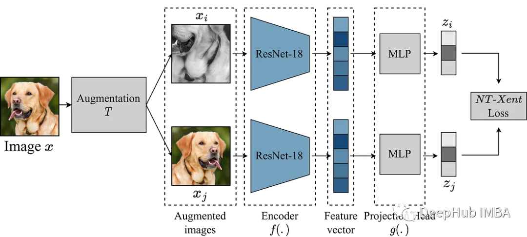
SimCLR 主要思想是通过增强模块 T 将图像与同一图像的其他增强版本进行对比，从而学习图像的良好表示。这是通过通过编码器网络 f(.) 映射图像，然后进行投影来完成的。 head g(.) 将学习到的特征映射到低维空间。然后在同一图像的两个增强版本的表示之间计算对比损失，以鼓励对同一图像的相似表示和对不同图像的不同表示。

本文我们将深入研究 SimCLR 框架并探索该算法的关键组件，包括数据增强、对比损失函数以及编码器和投影的head 架构。

我们这里使用来自 Kaggle 的垃圾分类数据集来进行实验

增强模块

SimCLR 中最重要的就是转换图像的增强模块。 SimCLR 论文的作者建议，强大的数据增强对于无监督学习很有用。因此，我们将遵循论文中推荐的方法。

调整大小的随机裁剪
50% 概率的随机水平翻转
随机颜色失真（颜色抖动概率为 80%，颜色下降概率为 20%）
50% 概率为随机高斯模糊

 defget_complete_transform(output_shape, kernel_size, s=1.0):
     """
     Color distortion transform
     
     Args:
         s: Strength parameter
         
     Returns:
         A color distortion transform
     """
     rnd_crop=RandomResizedCrop(output_shape)
     rnd_flip=RandomHorizontalFlip(p=0.5)
     
     color_jitter=ColorJitter(0.8*s, 0.8*s, 0.8*s, 0.2*s)
     rnd_color_jitter=RandomApply([color_jitter], p=0.8)
     
     rnd_gray=RandomGrayscale(p=0.2)
     gaussian_blur=GaussianBlur(kernel_size=kernel_size)
     rnd_gaussian_blur=RandomApply([gaussian_blur], p=0.5)
     to_tensor=ToTensor()
     image_transform=Compose([
         to_tensor,
         rnd_crop,
         rnd_flip,
         rnd_color_jitter,
         rnd_gray,
         rnd_gaussian_blur,
     ])
     returnimage_transform
 
 classContrastiveLearningViewGenerator(object):
     """
     Take 2 random crops of 1 image as the query and key.
     """
     def__init__(self, base_transform, n_views=2):
         self.base_transform=base_transform
         self.n_views=n_views
         
     def__call__(self, x):
         views= [self.base_transform(x) foriinrange(self.n_views)]
         returnviews

下一步就是定义一个PyTorch 的 Dataset 。

 classCustomDataset(Dataset):
     def__init__(self, list_images, transform=None):
         """
         Args:
             list_images (list): List of all the images
             transform (callable, optional): Optional transform to be applied on a sample.
         """
         self.list_images=list_images
         self.transform=transform
         
     def__len__(self):
         returnlen(self.list_images)
     
     def__getitem__(self, idx):
         iftorch.is_tensor(idx):
             idx=idx.tolist()
             
         img_name=self.list_images[idx]
         image=io.imread(img_name)
         ifself.transform:
             image=self.transform(image)
             
         returnimage

作为样例，我们使用比较小的模型 ResNet18 作为主干，所以他的输入是 224x224 图像，我们按照要求设置一些参数并生成dataloader

 out_shape= [224, 224]
 kernel_size= [21, 21] # 10% of out_shape
 
 # Custom transform
 base_transforms=get_complete_transform(output_shape=out_shape, kernel_size=kernel_size, s=1.0)
 custom_transform=ContrastiveLearningViewGenerator(base_transform=base_transforms)
 
 garbage_ds=CustomDataset(
     list_images=glob.glob("/kaggle/input/garbage-classification/garbage_classification/*/*.jpg"),
     transform=custom_transform
 )
 
 BATCH_SZ=128
 
 # Build DataLoader
 train_dl=torch.utils.data.DataLoader( 
     garbage_ds,
     batch_size=BATCH_SZ,
     shuffle=True,
     drop_last=True,
     pin_memory=True)

SimCLR

我们已经准备好了数据，开始对模型进行复现。上面的增强模块提供了图像的两个增强视图，它们通过编码器前向传递以获得相应的表示。 SimCLR 的目标是通过鼓励模型从两个不同的增强视图中学习对象的一般表示来最大化这些不同学习表示之间的相似性。

编码器网络的选择不受限制，可以是任何架构。上面已经说了，为了简单演示，我们使用 ResNet18。编码器模型学习到的表示决定了相似性系数，为了提高这些表示的质量，SimCLR 使用投影头将编码向量投影到更丰富的潜在空间中。这里我们将ResNet18的512维度的特征投影到256的空间中，看着很复杂，其实就是加了一个带relu的mlp。

 classIdentity(nn.Module):
     def__init__(self):
         super(Identity, self).__init__()
     defforward(self, x):
         returnx
     
 classSimCLR(nn.Module):
     def__init__(self, linear_eval=False):
         super().__init__()
         self.linear_eval=linear_eval
         resnet18=models.resnet18(pretrained=False)
         resnet18.fc=Identity()
         self.encoder=resnet18
         self.projection=nn.Sequential(
             nn.Linear(512, 512),
             nn.ReLU(),
             nn.Linear(512, 256)
         )
     defforward(self, x):
         ifnotself.linear_eval:
             x=torch.cat(x, dim=0)
         encoding=self.encoder(x)
         projection=self.projection(encoding)
         returnprojection

对比损失

对比损失函数，也称为归一化温度标度交叉熵损失 (NT-Xent)，是 SimCLR 的一个关键组成部分，它鼓励模型学习相同图像的相似表示和不同图像的不同表示。

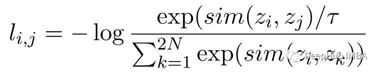
NT-Xent 损失是使用一对通过编码器网络传递的图像的增强视图来计算的，以获得它们相应的表示。对比损失的目标是鼓励同一图像的两个增强视图的表示相似，同时迫使不同图像的表示不相似。

NT-Xent 将 softmax 函数应用于增强视图表示的成对相似性。 softmax 函数应用于小批量内的所有表示对，得到每个图像的相似性概率分布。温度参数temperature 用于在应用 softmax 函数之前缩放成对相似性，这有助于在优化过程中获得更好的梯度。

在获得相似性的概率分布后，通过最大化同一图像的匹配表示的对数似然和最小化不同图像的不匹配表示的对数似然来计算 NT-Xent 损失。

 LABELS=torch.cat([torch.arange(BATCH_SZ) foriinrange(2)], dim=0)
 LABELS= (LABELS.unsqueeze(0) ==LABELS.unsqueeze(1)).float() #one-hot representations
 LABELS=LABELS.to(DEVICE)
 
 defntxent_loss(features, temp):
     """
     NT-Xent Loss.
     
     Args:
         z1: The learned representations from first branch of projection head
         z2: The learned representations from second branch of projection head 
     Returns:
         Loss
     """
     similarity_matrix=torch.matmul(features, features.T) 
     mask=torch.eye(LABELS.shape[0], dtype=torch.bool).to(DEVICE)
     labels=LABELS[~mask].view(LABELS.shape[0], -1)
     similarity_matrix=similarity_matrix[~mask].view(similarity_matrix.shape[0], -1)
     
     positives=similarity_matrix[labels.bool()].view(labels.shape[0], -1)
     
     negatives=similarity_matrix[~labels.bool()].view(similarity_matrix.shape[0], -1)
     
     logits=torch.cat([positives, negatives], dim=1)
     labels=torch.zeros(logits.shape[0], dtype=torch.long).to(DEVICE)
     
     logits=logits/temp
     returnlogits, labels

所有的准备都完成了，让我们训练 SimCLR 看看效果！

 simclr_model=SimCLR().to(DEVICE)
 criterion=nn.CrossEntropyLoss().to(DEVICE)
 optimizer=torch.optim.Adam(simclr_model.parameters())
 
 epochs=10
 withtqdm(total=epochs) aspbar:
     forepochinrange(epochs):
         t0=time.time()
         running_loss=0.0
         fori, viewsinenumerate(train_dl):
             projections=simclr_model([view.to(DEVICE) forviewinviews])
             logits, labels=ntxent_loss(projections, temp=2)
             loss=criterion(logits, labels)
             optimizer.zero_grad() 
             loss.backward()
             optimizer.step() 
             
             # print stats
             running_loss+=loss.item()
             ifi%10==9: # print every 10 mini-batches
                 print(f"Epoch: {epoch+1} Batch: {i+1} Loss: {(running_loss/100):.4f}")
                 running_loss=0.0
         pbar.update(1)
         print(f"Time taken: {((time.time()-t0)/60):.3f} mins")

上面代码训练了10轮，假设我们已经完成了预训练过程，可以将预训练的编码器用于我们想要的下游任务。这可以通过下面的代码来完成。

 fromtorchvision.transformsimportResize, CenterCrop
 resize=Resize(255)
 ccrop=CenterCrop(224)
 ttensor=ToTensor()
 
 custom_transform=Compose([
     resize,
     ccrop,
     ttensor,
 ])
 
 garbage_ds=ImageFolder(
     root="/kaggle/input/garbage-classification/garbage_classification/",
     transform=custom_transform
 )
 
 classes=len(garbage_ds.classes)
 
 BATCH_SZ=128
 
 train_dl=torch.utils.data.DataLoader(
     garbage_ds,
     batch_size=BATCH_SZ, 
     shuffle=True,
     drop_last=True,
     pin_memory=True,
 )
 
 classIdentity(nn.Module):
     def__init__(self):
         super(Identity, self).__init__() 
     defforward(self, x):
         returnx
     
 classLinearEvaluation(nn.Module):
     def__init__(self, model, classes):
         super().__init__()
         simclr=model
         simclr.linear_eval=True
         simclr.projection=Identity()
         self.simclr=simclr
         forparaminself.simclr.parameters():
             param.requires_grad=False
         self.linear=nn.Linear(512, classes)
     defforward(self, x):
         encoding=self.simclr(x)
         pred=self.linear(encoding)
         returnpred
       
 eval_model=LinearEvaluation(simclr_model, classes).to(DEVICE)
 criterion=nn.CrossEntropyLoss().to(DEVICE)
 optimizer=torch.optim.Adam(eval_model.parameters())
 
 preds, labels= [], []
 correct, total=0, 0
 
 withtorch.no_grad():
     t0=time.time()
     forimg, gtintqdm(train_dl):
         image=img.to(DEVICE)
         label=gt.to(DEVICE)
         pred=eval_model(image)
         _, pred=torch.max(pred.data, 1)
         total+=label.size(0)
         correct+= (pred==label).float().sum().item()
 
     print(f"Time taken: {((time.time()-t0)/60):.3f} mins")
     
 print(
         "Accuracy of the network on the {} Train images: {} %".format(
             total, 100*correct/total
         )
     )

上面的代码最主要的部分就是读取刚刚训练的simclr模型，然后冻结所有的权重，然后再创建一个分类头self.linear ，进行下游的分类任务

总结

本文介绍了SimCLR框架，并使用它来预训练随机初始化权重的ResNet18。预训练是深度学习中使用的一种强大的技术，用于在大型数据集上训练模型，学习可以转移到其他任务中的有用特征。SimCLR论文认为，批量越大，性能越好。我们的实现只使用128个批大小，只训练10个epoch。所以这不是模型的最佳性能，如果需要性能对比还需要进一步的训练。

论文地址：https://arxiv.org/abs/2002.05709 有兴趣的可以阅读

本文作者：Prabowo Yoga Wicaksana

标签：深度学习 pytorch 对比学习

使用Pytorch实现对比学习SimCLR 进行自监督预训练

增强模块

SimCLR

对比损失

总结

发表评论

“使用Pytorch实现对比学习SimCLR 进行自监督预训练”的评论:

关于作者

Deephub

相关阅读

文章导航