
在这篇文章中,我们将看到如何处理回归问题,以及如何通过使用特征转换、特征工程、聚类、增强算法等概念来提高机器学习模型的准确性。
数据科学是一个迭代的过程,只有经过反复的实验,我们才能得到最适合我们需求的模型/解决方案。

让我们通过一个例子来关注上面的每个阶段。我有一个健康保险数据集(CSV文件),其中包含保险费用、年龄、性别、BMI等客户信息。我们必须根据数据集中的这些参数预测保险费用。这是一个回归问题,因为我们的目标变量——费用/保险成本——是数字的。
让我们从加载数据集和探索属性开始(EDA -探索性数据分析)
 #Load csv into a dataframe
 df=pd.read_csv('insurance_data.csv')
 df.head(3)#Get the number of rows and columns
 print(f'Dataset size: {df.shape}')
 (1338,7)
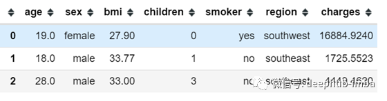
数据集有1338条记录和6个特性。吸烟者、性别和地区是分类变量,而年龄、BMI和儿童是数字变量。
零/缺失值处理
让我们检查数据集中缺失值的比例:
df.isnull().sum().sort_values(ascending=False)/df.shape[0]

年龄和BMI有一些零值——虽然很少。我们将处理这些缺失的数据,然后开始数据分析。Sklearn的SimpleImputer允许您根据各自列中的平均值/中值/最频繁值替换缺失的值。在本例中,我使用中值来填充空值。
 #Instantiate SimpleImputer
 si=SimpleImputer(missing_values = np.nan, strategy="median")
 si.fit(df[[’age’, 'bmi’]])

 #Filling missing data with median
 df[[’age’, 'bmi’]] = si.transform(df[[’age’, 'bmi’]])
数据可视化
现在我们的数据是干净的,我们将通过可视化和地图来分析数据。一个简单的海产配对可以给我们很多启示!
sns.pairplot(data=df, diag_kind='kde')
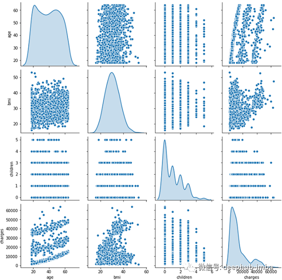
我们看到了什么?
收费和儿童被扭曲了。
年龄与收费呈正相关。
BMI服从正态分布!😎
Seaborn的箱线图和计数图可以用来揭示分类变量对收费的影响。

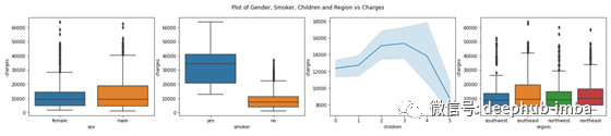
根据上述图的观察:
男性和女性的数量几乎相等,男性和女性的平均收费中位数也相同,但男性的收费范围更高。
吸烟者的保险费用相对较高。
有2-3个孩子的人收费最高
这4个地区的客户几乎是平均分布的,而且他们的费用几乎相同。
女性吸烟者的百分比低于男性吸烟者的百分比。
因此,我们可以得出结论,“吸烟者”对保险费用有相当大的影响,而性别的影响最小。
让我们创建一个热图来理解特征(年龄、BMI和儿童)之间的相关性。
 sns.heatmap(df[['age', 'bmi', 'children', 'charges']].corr(), cmap='Blues', annot=True)
 plt.show()

我们看到年龄和体重指数与收费有平均相关性。
现在,我们将逐一介绍模型准备和模型开发的步骤。
特征编码
在这个步骤中,我们将分类变量——吸烟者、性别和地区——转换为数字格式(0、1、2、3等),因为大多数算法不能处理非数字数据。这个过程叫做编码,有很多方法可以做到这一点:
LabelEncoding—将分类值表示为数字(例如,带有意大利、印度、美国、英国等值的Region可以表示为1、2、3、4)
OrdinalEncoding——用于将基于排名的分类数据值表示为数字。(例如用1,2,3表示高、中、低)
独热编码-将类别数据表示为二进制值-仅0和1。如果分类特性中没有很多唯一的值,我更喜欢使用独热编码而不是标签编码。在这里,我在Region上使用了pandas的一个编码函数(get_dummies),并将其分成4列——location_NE、location_SE、location_NW和location_SW。也可以在本专栏中使用标签编码,但是,独热编码给了我更好的结果。
 #One hot encoding
 region=pd.get_dummies(df.region, prefix='location')
 df = pd.concat([df,region],axis=1)
 df.drop(columns='region', inplace=True)df.sex.replace(to_replace=['male','female'],value=[1,0], inplace=True)
 df.smoker.replace(to_replace=['yes', 'no'], value=[1,0], inplace=True)
特征选择和缩放
接下来,我们将选择最能影响“收费”的功能。我选择了除“性别”以外的所有功能,因为它对收费的影响很小(从上面的图表得出结论)。这些特征将构成变量X,而费用将构成变量y。如果有很多特性,我建议您使用scikit-learn的SelectKBest进行特性选择,以到达顶级特性。
 #Feature Selection
 y=df.charges.values
 X=df[['age', 'bmi', 'smoker', 'children', 'location_northeast', 'location_northwest', 'location_southeast', 'location_southwest']]#Split data into test and train
 X_train, X_test, y_train, y_test=train_test_split(X,y, test_size=0.2, random_state=42)
一旦我们选择了我们的特征,我们需要“标准化”数字——年龄、BMI、儿童。标准化过程将数据转换为0到1范围内的更小的值,这样所有的值都处于相同的尺度上,而不是一个压倒另一个。我在这里使用了StandardScaler。
 #Scaling numeric features using sklearn StandardScalar
 numeric=['age', 'bmi', 'children']
 sc=StandardScalar()
 X_train[numeric]=sc.fit_transform(X_train[numeric])
 X_test[numeric]=sc.transform(X_test[numeric])
现在,我们已经准备好创建我们的第一个基本模型😀。我们将尝试线性回归和决策树来预测保险费用
 from sklearn.linear_model import LinearRegression
 from sklearn.tree import DecisionTreeRegressor
 from sklearn.metrics import r2_score, mean_absolute_error, mean_squared_error

 #Create a LinearRegression object
 lr= LinearRegression()
 #Fit X and y
 lr.fit(X_train, y_train)
 ypred = lr.predict(X_test)
 #Metrics to evaluate your model
 r2_score(y_test, ypred), mean_absolute_error(y_test, ypred), np.sqrt(mean_squared_error(y_test, ypred))


 dt = DecisionTreeRegressor()
 dt.fit(X_train, y_train)
 yhat = dt.predict(X_test)
 r2_score(y_test, yhat), mean_absolute_error(y_test, yhat), np.sqrt(mean_squared_error(y_test, yhat))

平均绝对误差(MAE)和均方根误差(RMSE)是用来评价回归模型的指标。你可以在这里阅读更多。我们的基线模型给出了超过76%的分数。在这两种方法之间,decision - trees给出的MAE更好为2780。
让我们看看如何使我们的模型更好。
特性工程
我们可以通过操纵数据集中的一些特征来提高模型得分。经过几次试验,我发现下面的项目可以提高准确性:
使用KMeans将类似的客户分组到集群中。
在区域栏中,将东北、西北区域划分为“北”区域,将东南、西南区域划分为“南”区域。
将' children '转换为一个名为' more_than_one_child '的分类特性,如果child的数量为> 1,则该特性为' Yes '
 from sklearn.cluster import KMeans
 features=['age', 'bmi', 'smoker', 'children', 'location_northeast', 'location_northwest', 'location_southeast', 'location_southwest']
 kmeans = KMeans(n_clusters=2)
 kmeans.fit(df[features])

 df['cust_type'] = kmeans.predict(df[features])

 df['location_north']=df.apply(lambda x: get_north(x['location_northeast'], x['location_northwest']), axis=1

 df['location_south']=df.apply(lambda x: get_south(x['location_southwest'], x['location_southeast']), axis=1)

 df['more_than_1_child']=df.children.apply(lambda x:1 if x>1 else 0)

特征转换
从我们的EDA,我们知道“费用”(Y)的分布是高度倾斜的,因此我们将应用scikit-learn的目标转换- QuantileTransformer来标准化这种行为。
 X=df[['age', 'bmi', 'smoker', 'more_than_1_child', 'cust_type', 'location_north', 'location_south']]

 #Split test and train data
 X_train, X_test, y_train, y_test=train_test_split(X,y, test_size=0.2, random_state=42)

 model = DecisionTreeRegressor()
 regr_trans = TransformedTargetRegressor(regressor=model, transformer=QuantileTransformer(output_distribution='normal'))
 regr_trans.fit(X_train, y_train)
 yhat = regr_trans.predict(X_test)
 round(r2_score(y_test, yhat), 3), round(mean_absolute_error(y_test, yhat), 2), round(np.sqrt(mean_squared_error(y_test, yhat)),2)

 >>0.843, 2189.28, 4931.96
哇,惊人的84%,MAE已经降到了2189!
使用集成和增强算法
现在我们将使用这些功能的集成基于随机森林,梯度增强,LightGBM,和XGBoost。如果你是一个初学者,没有意识到boosting 和bagging 的方法。
 X=df[['age', 'bmi', 'smoker', 'more_than_1_child', 'cust_type', 'location_north', 'location_south']]

 model = RandomForestRegressor()
 #transforming target variable through quantile transformer
 ttr = TransformedTargetRegressor(regressor=model, transformer=QuantileTransformer(output_distribution='normal'))
 ttr.fit(X_train, y_train)
 yhat = ttr.predict(X_test)

 r2_score(y_test, yhat), mean_absolute_error(y_test, yhat), np.sqrt(mean_squared_error(y_test, yhat))

 >>0.8802, 2078, 4312
是的!我们的随机森林模型表现很好- 2078的MAE👍。现在,我们将尝试一些增强算法,如梯度增强,LightGBM,和XGBoost。
 from sklearn.ensemble import GradientBoostingRegressor
 import lightgbm
 import xgboost

 #generic function to fit model and return metrics for every algorithm
 def boost_models(x):
     #transforming target variable through quantile transformer
     regr_trans = TransformedTargetRegressor(regressor=x, transformer=QuantileTransformer(output_distribution='normal'))
     regr_trans.fit(X_train, y_train)
     yhat = regr_trans.predict(X_test)
     algoname= x.__class__.__name__
     return algoname, round(r2_score(y_test, yhat),3), round(mean_absolute_error(y_test, yhat),2), round(np.sqrt(mean_squared_error(y_test, yhat)),2)

 algo=[GradientBoostingRegressor(), lgbm.LGBMRegressor(), xg.XGBRFRegressor()]
 score=[]
 for a in algo:
     score.append(boost_models(a))

  #Collate all scores in a table
  pd.DataFrame(score, columns=['Model', 'Score', 'MAE', 'RMSE'])
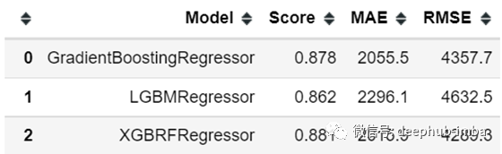
Hyperparameter调优
让我们调整一些算法参数,如树深度、估计值、学习率等,并检查模型的准确性。手动尝试参数值的不同组合非常耗时。Scikit-learn的GridSearchCV自动执行此过程,并计算这些参数的优化值。我已经将GridSearch应用于上述3种算法。下面是XGBoost的一个:
 from sklearn.model_selection import GridSearchCV

 param_grid = {'n_estimators': [100, 80, 60, 55, 51, 45],
               'max_depth': [7, 8],
               'reg_lambda' :[0.26, 0.25, 0.2]
              }

 grid = GridSearchCV(xg.XGBRFRegressor(), param_grid, refit = True, verbose = 3, n_jobs=-1) #
 regr_trans = TransformedTargetRegressor(regressor=grid, transformer=QuantileTransformer(output_distribution='normal'))

 # fitting the model for grid search
 grid_result=regr_trans.fit(X_train, y_train)
 best_params=grid_result.regressor_.best_params_
 print(best_params)

 #using best params to create and fit model
 best_model = xg.XGBRFRegressor(max_depth=best_params["max_depth"], n_estimators=best_params["n_estimators"], reg_lambda=best_params["reg_lambda"])
 regr_trans = TransformedTargetRegressor(regressor=best_model, transformer=QuantileTransformer(output_distribution='normal'))
 regr_trans.fit(X_train, y_train)
 yhat = regr_trans.predict(X_test)

 #evaluate metrics
 r2_score(y_test, yhat), mean_absolute_error(y_test, yhat), np.sqrt(mean_squared_error(y_test, yhat))

一旦我们得到了参数的最优值,我们将使用这些值再次运行所有3个模型。
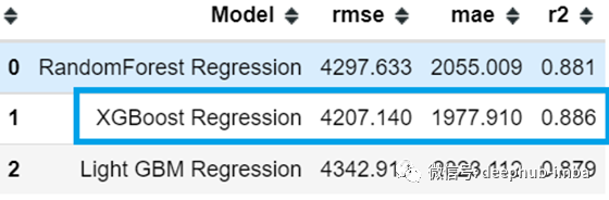
这个看起来好多了!我们已经能够提高我们的准确性- XGBoost给出了88.6%的分数,相对较少的错误

分布和残差图证实了预测费用和实际费用之间有很好的重叠。然而,有一些预测值远远超出了x轴,这使得我们的均方根误差更高。我们可以通过增加数据点(即收集更多数据)来减少这种情况。
现在我们已经准备好将这个模型部署到生产环境中,并在未知数据上对其进行测试。
简而言之,提高我模型准确性的要点
- 创建简单的新特征
- 转换目标变量
- 聚类公共数据点
- 使用增强算法
- Hyperparameter调优
你可以在这里找到我的笔记本。并不是所有的方法都适用于你的模型。挑选最适合你的方案:)
https://github.com/sacharya225/data-expts/tree/master/Health%20Insurance%20Cost%20Prediction
作者:Shwetha Acharya
本文地址:https://towardsdatascience.com/how-to-improve-the-accuracy-of-a-regression-model-3517accf8604
deephub翻译组