
点击上方“Deephub Imba”,关注公众号,好文章不错过 !
Isomap Embedding 等距特征映射是一种新颖,高效的非线性降维技术,它的一个突出优点是只有两个参数需要设定,即邻域参数和嵌入维数.
在文章中,我们讨论一下问题:
- Isomap 属于哪一类机器学习技术?
- Isomap 是如何工作的?我通过一个直观的例子而不是复杂的数学来解释。
- 如何使用 Isomap 减少数据的维度?
机器学习算法系列中的 Isomap
机器学习算法太多了,可能永远不可能将它们全部收集和分类。然而,我已经尝试为一些最常用的做这件事,你可以在下面的旭日图中找到这些👇。

图太大了可能的不太清楚,这几强调一下,Isomap 是一种旨在降维的无监督机器学习技术。
它与同一类别中的其他一些技术不同,它使用非线性降维方法而不是 PCA 等算法使用的线性映射。我们将在下一节中看到线性方法与非线性方法有何不同。
等距映射 (Isomap) 如何工作?
Isomap 是一种结合了几种不同算法的技术,使其能够使用非线性方式来减少维度,同时保留局部结构。
在我们查看 Isomap 的示例并将其与主成分分析 (PCA) 的线性方法进行比较之前,让我们列出 Isomap 执行步骤:
使用 KNN 方法找到每个数据点的 k 个最近邻。此处,“k”是可以在模型超参数中指定的邻居数量。
找到邻居后,如果点是彼此的邻居,则构建邻域图,其中点相互连接。不是邻居的数据点保持未连接状态。
计算每对数据点(节点)之间的最短路径。通常,用于此任务的是 Floyd-Warshall 或 Dijkstra 算法。请注意,此步骤通常也被描述为找到点之间的测地线距离。
使用多维缩放 (MDS) 计算低维嵌入。给定每对点之间的距离,MDS 将每个对象放入 N 维空间(N 被指定为超参数),以便尽可能保留点之间的距离。
对于我们的示例,让我们创建一个称为瑞士卷的 3D 对象。该对象由 2,000 个单独的数据点组成。

接下来,我们要使用 Isomap 将这个 3 维瑞士卷映射到 2 维。要跟踪此转换过程中发生的情况,让我们选择两个点:A 和 B。
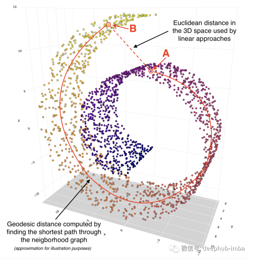
我们可以看到这两个点在 3D 空间内彼此相对靠近。如果我们使用诸如 PCA 之类的线性降维方法,那么这两个点之间的欧几里得距离在较低维度上会保持一些相似。请参阅下面的 PCA 转换图表:

请注意,PCA 中 2D 对象的形状看起来像是从特定角度拍摄的同一 3D 对象的图片。这是线性变换的一个特点。
同时,诸如 Isomap 之类的非线性方法给了我们非常不同的结果。我们可以将这种转换描述为展开瑞士卷并将其平放在 2D 表面上:

我们可以看到,二维空间中点 A 和 B 之间的距离基于通过邻域连接计算的测地线距离。
这就是 Isomap 能够执行非线性降维的秘诀,它专注于保留局部结构而较少关注全局结构。
如何使用 Isomap ?
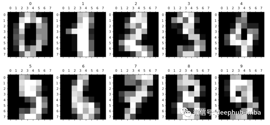
现在让我们使用 Isomap 来降低 MNIST 数据集(手写数字集合)中图片的高维数。这将使我们能够看到不同的数字如何在 3D 空间中聚集在一起。
设置我们将使用以下数据和库:
- Scikit-learn
- Plotly 和 Matplotlib
- Pandas
让我们导入库。
 import pandas as pd # for data manipulation

 # Visualization
 import plotly.express as px # for data visualization
 import matplotlib.pyplot as plt # for showing handwritten digits

 # Skleran
 from sklearn.datasets import load_digits # for MNIST data
 from sklearn.manifold import Isomap # for Isomap dimensionality reduction
接下来,我们加载 MNIST 数据。
 # Load digits data
 digits = load_digits()

 # Load arrays containing digit data (64 pixels per image) and their true labels
 X, y = load_digits(return_X_y=True)

 # Some stats
 print('Shape of digit images: ', digits.images.shape)
 print('Shape of X (training data): ', X.shape)
 print('Shape of y (true labels): ', y.shape)

让我们显示前 10 个手写数字,以便更好地了解我们正在处理的内容。
 # Display images of the first 10 digits
 fig, axs = plt.subplots(2, 5, sharey=False, tight_layout=True, figsize=(12,6), facecolor='white')
 n=0
 plt.gray()
 for i in range(0,2):
     for j in range(0,5):
         axs[i,j].matshow(digits.images[n])
         axs[i,j].set(title=y[n])
         n=n+1
 plt.show()
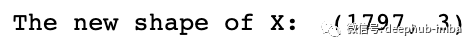
我们现在将应用 Isomap 将 X 数组中每条记录的维数从 64 减少到 3。
 ### Step 1 - Configure the Isomap function, note we use default hyperparameter values in this example
 embed3 = Isomap(
     n_neighbors=5, # default=5, algorithm finds local structures based on the nearest neighbors
     n_components=3, # number of dimensions
     eigen_solver='auto', # {‘auto’, ‘arpack’, ‘dense’}, default=’auto’
     tol=0, # default=0, Convergence tolerance passed to arpack or lobpcg. not used if eigen_solver == ‘dense’.
     max_iter=None, # default=None, Maximum number of iterations for the arpack solver. not used if eigen_solver == ‘dense’.
     path_method='auto', # {‘auto’, ‘FW’, ‘D’}, default=’auto’, Method to use in finding shortest path.
     neighbors_algorithm='auto', # neighbors_algorithm{‘auto’, ‘brute’, ‘kd_tree’, ‘ball_tree’}, default=’auto’
     n_jobs=-1, # n_jobsint or None, default=None, The number of parallel jobs to run. -1 means using all processors
     metric='minkowski', # string, or callable, default=”minkowski”
     p=2, # default=2, Parameter for the Minkowski metric. When p = 1, this is equivalent to using manhattan_distance (l1), and euclidean_distance (l2) for p = 2
     metric_params=None # default=None, Additional keyword arguments for the metric function.
 )

 ### Step 2 - Fit the data and transform it, so we have 3 dimensions instead of 64
 X_trans3 = embed3.fit_transform(X)

 ### Step 3 - Print shape to test
 print('The new shape of X: ',X_trans3.shape)
最后,让我们绘制一个 3D 散点图,看看将维度降低到 3 后数据的样子。
 # Create a 3D scatter plot
 fig = px.scatter_3d(None,
                     x=X_trans3[:,0], y=X_trans3[:,1], z=X_trans3[:,2],
                     color=y.astype(str),
                     height=900, width=900
                    )

 # Update chart looks
 fig.update_layout(#title_text="Scatter 3D Plot",
                   showlegend=True,
                   legend=dict(orientation="h", yanchor="top", y=0, xanchor="center", x=0.5),
                   scene_camera=dict(up=dict(x=0, y=0, z=1),
                                         center=dict(x=0, y=0, z=-0.2),
                                         eye=dict(x=-1.5, y=1.5, z=0.5)),
                                         margin=dict(l=0, r=0, b=0, t=0),
                   scene = dict(xaxis=dict(backgroundcolor='white',
                                           color='black',
                                           gridcolor='#f0f0f0',
                                           title_font=dict(size=10),
                                           tickfont=dict(size=10),
                                          ),
                                yaxis=dict(backgroundcolor='white',
                                           color='black',
                                           gridcolor='#f0f0f0',
                                           title_font=dict(size=10),
                                           tickfont=dict(size=10),
                                           ),
                                zaxis=dict(backgroundcolor='lightgrey',
                                           color='black',
                                           gridcolor='#f0f0f0',
                                           title_font=dict(size=10),
                                           tickfont=dict(size=10),
                                          )))

 # Update marker size
 fig.update_traces(marker=dict(size=2))

 fig.show()
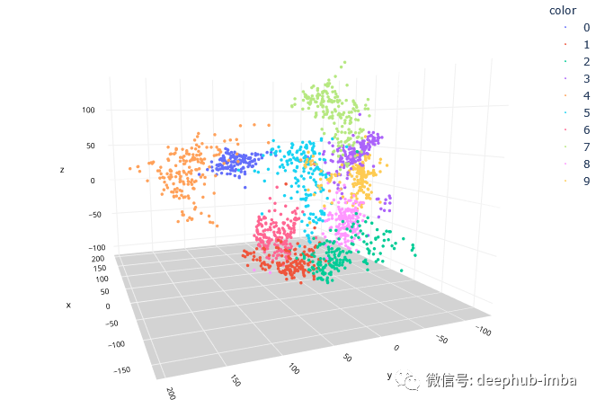
Isomap 在将维度从 64 减少到 3 方面做得非常出色,同时保留了非线性关系。这使我们能够在 3 维空间中可视化手写数字的簇。
对于机器学习的下一步,我们现在可以轻松使用决策树、SVM 或 KNN 等分类模型之一来预测每个手写数字标签。
总结
Isomap 是降维的最佳工具之一,使我们能够保留数据点之间的非线性关系。
我们已经看到了 Isomap 算法如何在实践中用于手写数字识别。同样,您可以使用 Isomap 作为 NLP(自然语言处理)分析的一部分,以在训练分类模型之前减少文本数据的高维。
我希望这篇文章能让你轻松了解 Isomap 的工作原理及其在数据科学项目中的优势。
如果您有任何问题或建议,请随时与我们联系。
作者:Saul Dobilas
喜欢就关注一下吧:
点个 在看 你最好看!********** **********