目标检测模型SSD的详细解释

目标检测由两个独立的任务组成，即分类和定位。R-CNN 系列目标检测器由两个阶段组成，分别是区域提议网络和分类和框细化头。然而，这种2阶段的检测模型已经基本被单阶段的模型替代了。在本文中，我想介绍 Single Shot MultiBox Detector (SSD)。

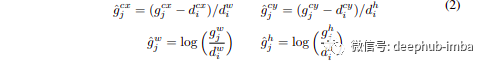
边界框回归

与 Faster R-CNN 一样，作者回归到默认边界框 (d) 的中心 (cx, cy) 及其宽度 (w) 和高度 (h) 的偏移量。因此，公式如下所示：

架构

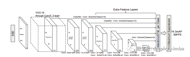
上图展示了基于 VGG-16 作为主干的架构。我将通过将其分解为 3 个部分来解释该架构：主干、辅助卷积和预测卷积。为了您的方便，我还将提供一些代码。

基础网络

class VGGBase(nn.Module):
    """
    VGG base convolutions to produce lower-level feature maps.
    """
    def __init__(self):
        super(VGGBase, self).__init__()
        # Standard convolutional layers in VGG16
        self.conv1_1 = nn.Conv2d(3, 64, kernel_size=3, padding=1)  # stride = 1, by default
        self.conv1_2 = nn.Conv2d(64, 64, kernel_size=3, padding=1)
        self.pool1 = nn.MaxPool2d(kernel_size=2, stride=2)
        self.conv2_1 = nn.Conv2d(64, 128, kernel_size=3, padding=1)
        self.conv2_2 = nn.Conv2d(128, 128, kernel_size=3, padding=1)
        self.pool2 = nn.MaxPool2d(kernel_size=2, stride=2)
        self.conv3_1 = nn.Conv2d(128, 256, kernel_size=3, padding=1)
        self.conv3_2 = nn.Conv2d(256, 256, kernel_size=3, padding=1)
        self.conv3_3 = nn.Conv2d(256, 256, kernel_size=3, padding=1)
        self.pool3 = nn.MaxPool2d(kernel_size=2, stride=2, ceil_mode=True)  # ceiling (not floor) here for even dims
        self.conv4_1 = nn.Conv2d(256, 512, kernel_size=3, padding=1)
        self.conv4_2 = nn.Conv2d(512, 512, kernel_size=3, padding=1)
        self.conv4_3 = nn.Conv2d(512, 512, kernel_size=3, padding=1)
        self.pool4 = nn.MaxPool2d(kernel_size=2, stride=2)
        self.conv5_1 = nn.Conv2d(512, 512, kernel_size=3, padding=1)
        self.conv5_2 = nn.Conv2d(512, 512, kernel_size=3, padding=1)
        self.conv5_3 = nn.Conv2d(512, 512, kernel_size=3, padding=1)
        self.pool5 = nn.MaxPool2d(kernel_size=3, stride=1, padding=1)  # retains size because stride is 1 (and padding)
        # Replacements for FC6 and FC7 in VGG16
        self.conv6 = nn.Conv2d(512, 1024, kernel_size=3, padding=6, dilation=6)  # atrous convolution
        self.conv7 = nn.Conv2d(1024, 1024, kernel_size=1)
        # Load pretrained layers
        self.load_pretrained_layers()
    def forward(self, image):
        """
        Forward propagation.
        :param image: images, a tensor of dimensions (N, 3, 300, 300)
        :return: lower-level feature maps conv4_3 and conv7
        """
        out = F.relu(self.conv1_1(image))  # (N, 64, 300, 300)
        out = F.relu(self.conv1_2(out))  # (N, 64, 300, 300)
        out = self.pool1(out)  # (N, 64, 150, 150)
        out = F.relu(self.conv2_1(out))  # (N, 128, 150, 150)
        out = F.relu(self.conv2_2(out))  # (N, 128, 150, 150)
        out = self.pool2(out)  # (N, 128, 75, 75)
        out = F.relu(self.conv3_1(out))  # (N, 256, 75, 75)
        out = F.relu(self.conv3_2(out))  # (N, 256, 75, 75)
        out = F.relu(self.conv3_3(out))  # (N, 256, 75, 75)
        out = self.pool3(out)  # (N, 256, 38, 38), it would have been 37 if not for ceil_mode = True
        out = F.relu(self.conv4_1(out))  # (N, 512, 38, 38)
        out = F.relu(self.conv4_2(out))  # (N, 512, 38, 38)
        out = F.relu(self.conv4_3(out))  # (N, 512, 38, 38)
        conv4_3_feats = out  # (N, 512, 38, 38)
        out = self.pool4(out)  # (N, 512, 19, 19)
        out = F.relu(self.conv5_1(out))  # (N, 512, 19, 19)
        out = F.relu(self.conv5_2(out))  # (N, 512, 19, 19)
        out = F.relu(self.conv5_3(out))  # (N, 512, 19, 19)
        out = self.pool5(out)  # (N, 512, 19, 19), pool5 does not reduce dimensions
        out = F.relu(self.conv6(out))  # (N, 1024, 19, 19)
        conv7_feats = F.relu(self.conv7(out))  # (N, 1024, 19, 19)
        # Lower-level feature maps
        return conv4_3_feats, conv7_feats

我想强调的是，以下示例是在假设输入图像的大小为 300 x 300 的情况下提供的，如原始论文中所示。

可以看出，我们正在使用一个简单且众所周知的 VGG-16 网络来提取 conv4_3 和 conv7 的特征。此外，我们可以注意到特征维度分别为 (N, 512, 38, 38) 和 (N, 1024, 19, 19)。我希望这部分足够简单明了，可以继续讨论 Axuliary Convolutions

Auxiliary Convolutions

class AuxiliaryConvolutions(nn.Module):
    def __init__(self):
        super(AuxiliaryConvolutions, self).__init__()
        #input (N, 1024, 19, 19) that is conv7_feats
        # Auxiliary/additional convolutions on top of the VGG base
        self.conv8_1 = nn.Conv2d(1024, 256, kernel_size=1, padding=0)  # stride = 1, by default
        self.conv8_2 = nn.Conv2d(256, 512, kernel_size=3, stride=2, padding=1)  # dim. reduction because stride > 1
        self.conv9_1 = nn.Conv2d(512, 128, kernel_size=1, padding=0)
        self.conv9_2 = nn.Conv2d(128, 256, kernel_size=3, stride=2, padding=1)  # dim. reduction because stride > 1
        self.conv10_1 = nn.Conv2d(256, 128, kernel_size=1, padding=0)
        self.conv10_2 = nn.Conv2d(128, 256, kernel_size=3, padding=0)  # dim. reduction because padding = 0
        self.conv11_1 = nn.Conv2d(256, 128, kernel_size=1, padding=0)
        self.conv11_2 = nn.Conv2d(128, 256, kernel_size=3, padding=0)  # dim. reduction because padding = 0
        # Initialize convolutions' parameters
        self.init_conv2d()
    def init_conv2d(self):
        """
        Initialize convolution parameters using xavier initialization.
        """
        for c in self.children():
            if isinstance(c, nn.Conv2d):
                nn.init.xavier_uniform_(c.weight)
                nn.init.constant_(c.bias, 0.)
    def forward(self, conv7_feats):
        """
        Forward propagation.
        :param conv7_feats: lower-level conv7 feature map, a tensor of dimensions (N, 1024, 19, 19)
        :return: higher-level feature maps (N, 512, 10, 10), (N, 256, 5, 5), (N, 256, 3, 3) and (N, 256, 1, 1)
        """
        out = F.relu(self.conv8_1(conv7_feats))  # (N, 256, 19, 19)
        out = F.relu(self.conv8_2(out))  # (N, 512, 10, 10)
        conv8_2_feats = out  # (N, 512, 10, 10)
        out = F.relu(self.conv9_1(out))  # (N, 128, 10, 10)
        out = F.relu(self.conv9_2(out))  # (N, 256, 5, 5)
        conv9_2_feats = out  # (N, 256, 5, 5)
        out = F.relu(self.conv10_1(out))  # (N, 128, 5, 5)
        out = F.relu(self.conv10_2(out))  # (N, 256, 3, 3)
        conv10_2_feats = out  # (N, 256, 3, 3)
        out = F.relu(self.conv11_1(out))  # (N, 128, 3, 3)
        conv11_2_feats = F.relu(self.conv11_2(out))  # (N, 256, 1, 1)
        # Higher-level feature maps
        return conv8_2_feats, conv9_2_feats, conv10_2_feats, conv11_2_feats

Auxiliary Convolutions使我们能够在基础 VGG-16 网络之上获得附加功能。这些层的大小逐渐减小，并允许在多个尺度上进行检测预测。因此，我们传入网络的输入是从 VGG-16 网络获得的 conv7 特征。正如在应用卷积和 ReLU 激活函数时所看到的，我们应该保留中间特征，即 conv8_2、conv9_2、conv10_2 和 conv11_2。请花点时间查看代码和特征图的尺寸:)

选择默认边界框

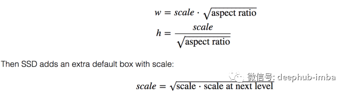
这听起来可能很可怕，但不要担心，它仍然很容易掌握。默认边界框是手动选择的。每个特征图层都分配了一个比例值。例如，Conv4_3 以 0.2（有时为 0.1）的最小尺度检测对象，然后线性增加到 conv11_2（从辅助卷积获得）的 0.9 尺度。此外，我们可以注意到，我们正在考虑每个特征图中每个位置的定义数量的先验框。对于进行 4 次预测的层，SSD 使用 4 种不同的纵横比，分别为 1、2、0.5 和 sqrt(s_k * s_(k+1))，其中 s_k 是第 k 个特征图的比例值。一般定义为长宽比为1时计算出的附加比例，然后默认框的宽高计算如下：

现在，让我们用以下代码对其进行总结。

def create_prior_boxes(self):
        """
        Create the 8732 prior (default) boxes for the SSD300, as defined in the paper.
    
        :return: prior boxes in center-size coordinates, a tensor of dimensions (8732, 4)
        """
        fmap_dims = {'conv4_3': 38,
                     'conv7': 19,
                     'conv8_2': 10,
                     'conv9_2': 5,
                     'conv10_2': 3,
                     'conv11_2': 1}
    
        obj_scales = {'conv4_3': 0.1,
                      'conv7': 0.2,
                      'conv8_2': 0.375,
                      'conv9_2': 0.55,
                      'conv10_2': 0.725,
                      'conv11_2': 0.9}
        """
        Note that we were considering four boxes in certain layers and six boxes in another layer. Now, if we want to
        have four boxes, we remove the {3, 1/3} aspect ratios, else we consider all of the six possible boxes
        """
        aspect_ratios = {'conv4_3': [1., 2., 0.5],
                         'conv7': [1., 2., 3., 0.5, .333],
                         'conv8_2': [1., 2., 3., 0.5, .333],
                         'conv9_2': [1., 2., 3., 0.5, .333],
                         'conv10_2': [1., 2., 0.5],
                         'conv11_2': [1., 2., 0.5]}
    
        fmaps = list(fmap_dims.keys())
    
        prior_boxes = []
        self.prior_boxes_info = []
    
        for k, fmap in enumerate(fmaps):
            for i in range(fmap_dims[fmap]):
                for j in range(fmap_dims[fmap]):
                    cx = (j + 0.5) / fmap_dims[fmap]
                    cy = (i + 0.5) / fmap_dims[fmap]
    
                    for ratio in aspect_ratios[fmap]:
                        prior_boxes.append([cx, cy, obj_scales[fmap] * sqrt(ratio), obj_scales[fmap] / sqrt(ratio)])
                        self.prior_boxes_info.append([fmap, i, j, ratio])
    
                        # For an aspect ratio of 1, use an additional prior whose scale is the geometric mean of the
                        # scale of the current feature map and the scale of the next feature map
                        if ratio == 1.:
                            try:
                                additional_scale = sqrt(obj_scales[fmap] * obj_scales[fmaps[k + 1]])
                            # For the last feature map, there is no "next" feature map
                            except IndexError:
                                additional_scale = 1.
                            prior_boxes.append([cx, cy, additional_scale, additional_scale])
                            self.prior_boxes_info.append([fmap, i, j, ratio])
    
        prior_boxes = torch.FloatTensor(prior_boxes).to(self.device)  # (8732, 4)
        prior_boxes.clamp_(0, 1)  # (8732, 4)
        return prior_boxes

它为 SSD 做出的 8732 个预测返回 8732 个先验框。

预测卷积

class PredictionConvolutions(nn.Module):
    """
    Convolutions to predict class scores and bounding boxes using lower and higher-level feature maps.
    The bounding boxes are predicted as encoded offsets w.r.t each of the 8732 anchor boxes.
    See 'cxcy_to_gcxgcy' in utils.py for the encoding definition.
    The class scores represent the scores of each object class in each of the 8732 bounding boxes located.
    A high score for 'background' = no object.
    """
    def __init__(self, n_classes):
        """
        :param n_classes: number of different types of objects
        """
        super(PredictionConvolutions, self).__init__()
        self.n_classes = n_classes
        # Number of prior-boxes we are considering per position in each feature map
        n_boxes = {'conv4_3': 4,
                   'conv7': 6,
                   'conv8_2': 6,
                   'conv9_2': 6,
                   'conv10_2': 4,
                   'conv11_2': 4}
        # 4 prior-boxes implies we use 4 different aspect ratios, etc.
        # Localization prediction convolutions (predict offsets w.r.t prior-boxes)
        self.loc_conv4_3 = nn.Conv2d(512, n_boxes['conv4_3'] * 4, kernel_size=3, padding=1)
        self.loc_conv7 = nn.Conv2d(1024, n_boxes['conv7'] * 4, kernel_size=3, padding=1)
        self.loc_conv8_2 = nn.Conv2d(512, n_boxes['conv8_2'] * 4, kernel_size=3, padding=1)
        self.loc_conv9_2 = nn.Conv2d(256, n_boxes['conv9_2'] * 4, kernel_size=3, padding=1)
        self.loc_conv10_2 = nn.Conv2d(256, n_boxes['conv10_2'] * 4, kernel_size=3, padding=1)
        self.loc_conv11_2 = nn.Conv2d(256, n_boxes['conv11_2'] * 4, kernel_size=3, padding=1)
        # Class prediction convolutions (predict classes in localization boxes)
        self.cl_conv4_3 = nn.Conv2d(512, n_boxes['conv4_3'] * n_classes, kernel_size=3, padding=1)
        self.cl_conv7 = nn.Conv2d(1024, n_boxes['conv7'] * n_classes, kernel_size=3, padding=1)
        self.cl_conv8_2 = nn.Conv2d(512, n_boxes['conv8_2'] * n_classes, kernel_size=3, padding=1)
        self.cl_conv9_2 = nn.Conv2d(256, n_boxes['conv9_2'] * n_classes, kernel_size=3, padding=1)
        self.cl_conv10_2 = nn.Conv2d(256, n_boxes['conv10_2'] * n_classes, kernel_size=3, padding=1)
        self.cl_conv11_2 = nn.Conv2d(256, n_boxes['conv11_2'] * n_classes, kernel_size=3, padding=1)
        # Initialize convolutions' parameters
        self.init_conv2d()
    def init_conv2d(self):
        """
        Initialize convolution parameters using xavier initialization.
        """
        for c in self.children():
            if isinstance(c, nn.Conv2d):
                nn.init.xavier_uniform_(c.weight)
                nn.init.constant_(c.bias, 0.)
    def forward(self, conv4_3_feats, conv7_feats, conv8_2_feats, conv9_2_feats, conv10_2_feats, conv11_2_feats):
    
           batch_size = conv4_3_feats.size(0)
           #predict boxes
           l_conv4_3 = self.loc_conv4_3(conv4_3_feats)  # (N, 16, 38, 38)
           l_conv4_3 = l_conv4_3.permute(0, 2, 3, 1).contiguous()  # (N, 38, 38, 16)
           l_conv4_3 = l_conv4_3.view(batch_size, -1, 4)  # (N, 5776, 4), there are a total 5776 boxes on this feature map
       
           l_conv7 = self.loc_conv7(conv7_feats)  # (N, 24, 19, 19)
           l_conv7 = l_conv7.permute(0, 2, 3, 1).contiguous()  # (N, 19, 19, 24)
           l_conv7 = l_conv7.view(batch_size, -1, 4)  # (N, 2166, 4)
       
           l_conv8_2 = self.loc_conv8_2(conv8_2_feats)  # (N, 24, 10, 10)
           l_conv8_2 = l_conv8_2.permute(0, 2, 3, 1).contiguous()  # (N, 10, 10, 24)
           l_conv8_2 = l_conv8_2.view(batch_size, -1, 4)  # (N, 600, 4)
       
           l_conv9_2 = self.loc_conv9_2(conv9_2_feats)  # (N, 24, 5, 5)
           l_conv9_2 = l_conv9_2.permute(0, 2, 3, 1).contiguous()  # (N, 5, 5, 24)
           l_conv9_2 = l_conv9_2.view(batch_size, -1, 4)  # (N, 150, 4)
       
           l_conv10_2 = self.loc_conv10_2(conv10_2_feats)  # (N, 16, 3, 3)
           l_conv10_2 = l_conv10_2.permute(0, 2, 3, 1).contiguous()  # (N, 3, 3, 16)
           l_conv10_2 = l_conv10_2.view(batch_size, -1, 4)  # (N, 36, 4)
       
           l_conv11_2 = self.loc_conv11_2(conv11_2_feats)  # (N, 16, 1, 1)
           l_conv11_2 = l_conv11_2.permute(0, 2, 3, 1).contiguous()  # (N, 1, 1, 16)
           l_conv11_2 = l_conv11_2.view(batch_size, -1, 4)  # (N, 4, 4)
       
           # Predict classes
           c_conv4_3 = self.cl_conv4_3(conv4_3_feats)  # (N, 4 * n_classes, 38, 38)
           c_conv4_3 = c_conv4_3.permute(0, 2, 3, 1).contiguous()  # (N, 38, 38, 4 * n_classes)
           c_conv4_3 = c_conv4_3.view(batch_size, -1, self.n_classes)  # (N, 5776, n_classes), there are a total 5776 boxes on this feature map
       
           c_conv7 = self.cl_conv7(conv7_feats)  # (N, 6 * n_classes, 19, 19)
           c_conv7 = c_conv7.permute(0, 2, 3, 1).contiguous()  # (N, 19, 19, 6 * n_classes)
           c_conv7 = c_conv7.view(batch_size, -1, self.n_classes)  # (N, 2166, n_classes)
       
           c_conv8_2 = self.cl_conv8_2(conv8_2_feats)  # (N, 6 * n_classes, 10, 10)
           c_conv8_2 = c_conv8_2.permute(0, 2, 3, 1).contiguous()  # (N, 10, 10, 6 * n_classes)
           c_conv8_2 = c_conv8_2.view(batch_size, -1, self.n_classes)  # (N, 600, n_classes)
       
           c_conv9_2 = self.cl_conv9_2(conv9_2_feats)  # (N, 6 * n_classes, 5, 5)
           c_conv9_2 = c_conv9_2.permute(0, 2, 3, 1).contiguous()  # (N, 5, 5, 6 * n_classes)
           c_conv9_2 = c_conv9_2.view(batch_size, -1, self.n_classes)  # (N, 150, n_classes)
       
           c_conv10_2 = self.cl_conv10_2(conv10_2_feats)  # (N, 4 * n_classes, 3, 3)
           c_conv10_2 = c_conv10_2.permute(0, 2, 3, 1).contiguous()  # (N, 3, 3, 4 * n_classes)
           c_conv10_2 = c_conv10_2.view(batch_size, -1, self.n_classes)  # (N, 36, n_classes)
       
           c_conv11_2 = self.cl_conv11_2(conv11_2_feats)  # (N, 4 * n_classes, 1, 1)
           c_conv11_2 = c_conv11_2.permute(0, 2, 3, 1).contiguous()  # (N, 1, 1, 4 * n_classes)
           c_conv11_2 = c_conv11_2.view(batch_size, -1, self.n_classes)  # (N, 4, n_classes)
       
           # A total of 8732 boxes
           # Concatenate in this specific order 
           locs = torch.cat([l_conv4_3, l_conv7, l_conv8_2, l_conv9_2, l_conv10_2, l_conv11_2], dim=1)  # (N, 8732, 4)
           classes_scores = torch.cat([c_conv4_3, c_conv7, c_conv8_2, c_conv9_2, c_conv10_2, c_conv11_2], dim=1)  # (N, 8732, n_classes)
       
           return locs, classes_scores

这可能看起来很复杂，但它基本上获得了我们从基础 VGG-16 和辅助卷积中获得的所有特征图，并应用卷积层来预测每个特征图的类别和边界框。

组合成完整代码

现在让我们把它们放在一起，看看最终的架构，如下所示。

class SSD300(nn.Module):
    """
    The SSD300 network - encapsulates the base VGG network, auxiliary, and prediction convolutions.
    """
    
    def __init__(self, n_classes, device):
        super(SSD300, self).__init__()
    
        self.n_classes = n_classes
        self.device = device
        self.base = VGGBase()
        self.aux_convs = AuxiliaryConvolutions()
        self.pred_convs = PredictionConvolutions(n_classes)
    
        # Since lower level features (conv4_3_feats) have considerably larger scales, we take the L2 norm and rescale
        # Rescale factor is initially set at 20, but is learned for each channel during back-prop
        self.rescale_factors = nn.Parameter(torch.FloatTensor(1, 512, 1, 1))  # there are 512 channels in conv4_3_feats
        nn.init.constant_(self.rescale_factors, 20)
    
        # Prior boxes
        self.priors_cxcy = self.create_prior_boxes()
        self.to(device)
    def forward(self, image):
      """
      Forward propagation.
      :param image: images, a tensor of dimensions (N, 3, 300, 300)
      :return: 8732 locations and class scores (i.e. w.r.t each prior box) for each image
      """
      # Run VGG base network convolutions 
      conv4_3_feats, conv7_feats = self.base(image)  # (N, 512, 38, 38), (N, 1024, 19, 19)
      # Rescale conv4_3 after L2 norm
      norm = conv4_3_feats.pow(2).sum(dim=1, keepdim=True).sqrt()  # (N, 1, 38, 38)
      conv4_3_feats = conv4_3_feats / norm  # (N, 512, 38, 38)
      conv4_3_feats = conv4_3_feats * self.rescale_factors  # (N, 512, 38, 38)
      # Run auxiliary convolutions
       # (N, 512, 10, 10),  (N, 256, 5, 5), (N, 256, 3, 3), (N, 256, 1, 1)
      conv8_2_feats, conv9_2_feats, conv10_2_feats, conv11_2_feats = self.aux_convs(conv7_feats) 
      # Run prediction convolutions
      # (N, 8732, 4), (N, 8732, n_classes)
      locs, classes_scores = self.pred_convs(conv4_3_feats, conv7_feats, conv8_2_feats, conv9_2_feats, conv10_2_feats, conv11_2_feats)  
      return locs, classes_scores

请注意，较低级别的特征（conv4_3_feats）具有相当大的尺度，因此我们采用 L2 范数并重新调整它。重新缩放因子最初设置为 20，但在反向传播期间为每个通道学习。

损失函数

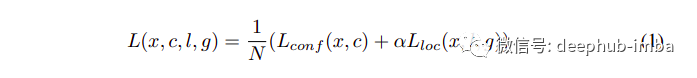
可以看出， 定位损失是 L1 平滑损失，而分类损失是众所周知的交叉熵损失。

匹配策略

在训练期间，我们需要确定哪些生成的先验框应该与我们要包含在损失计算中的地面实况框相对应。因此，我们将每个真实框与具有最高 Jaccard 重叠的先验框进行匹配。此外，我们还选择了重叠至少为 0.5 的先验框，以允许网络预测多个重叠框的高分。

在匹配步骤之后，大多数先验/默认框用作负样本。然而，为了避免正负样本之间的不平衡，我们最多保持 3:1 的比例，因为这样可以更快地优化和稳定学习。再一次，定位损失仅在正（非背景）先验上计算。

最后总结

我希望我设法使 SSD 易于理解和掌握。我尝试使用代码，以便您能够将过程可视化。花点时间去理解它。此外，如果您尝试自己使用它会更好。下次我将写关于 YOLO 系列物体检测器的文章。

作者：Chingis Oinar

原文地址：https://medium.com/mlearning-ai/object-detection-explained-single-shot-multibox-detector-c45e6a7af40