
在快速发展的自然语言处理领域,Transformers 已经成为主导模型,在广泛的序列建模任务中表现出卓越的性能,包括词性标记、命名实体识别和分块。在Transformers之前,条件随机场(CRFs)是序列建模的首选工具,特别是线性链CRFs,它将序列建模为有向图,而CRFs更普遍地可以用于任意图。
本文中crf的实现并不是最有效的实现,也缺乏批处理功能,但是它相对容易阅读和理解,因为本文的目的是让我们了解crf的内部工作,所以它非常适合我们。
发射和转换分数
在序列标记问题中,我们处理输入数据元素的序列,例如句子中的单词,其中每个元素对应于一个特定的标签或类别。目标是为每个单独的元素正确地分配适当的标签。在CRF-LSTM模型中,可以确定两个关键组成部分:发射和跃迁概率。我们实际上将处理对数空间中的分数,而不是数值稳定性的概率:
发射分数(Emission scores),神经网络输出的各个Tag的置信度
它与观察给定数据元素的特定标签的可能性有关。例如在命名实体识别的上下文中,序列中的每个单词都与三个标签中的一个相关联:实体的开头(B),实体的中间单词(I)或任何实体之外的单词(O)。发射概率量化了特定单词与特定标签相关联的概率。这在数学上表示为P(y_i | x_i),其中y_i表示标签,x_i表示输入单词。
转换分数(Transition scores),又叫过渡分数,描述了序列中从一个标签转换到另一个标签的可能性,也就是CRF层中各个Tag之间的转换概率
这些分数支持对连续标签之间的依赖关系进行建模。通过捕获这些依赖关系,转换分数有助于预测标签序列的连贯性和一致性。它们表示为P(y_i | y*(i-1)),其中y_i表示当前标签,y*(i-1)表示序列中的前一个标签。
这两个组件的协同作用产生了一个鲁棒的序列标记模型。
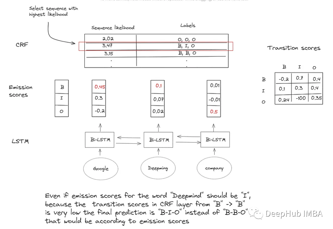
为了给给定的单词分配发射分数,可以使用各种特征函数,比如单词的上下文、它的形状(如大写模式,如果一个单词以大写字母开头,而不是在句子的开头,那么它很可能是一个实体的开头),形态学特征(包括前缀、后缀和词干)等等。定义这些特性可能是一项劳动密集型且耗时的工作。这就是为什么许多从业者选择双向LSTM模型,它可以根据每个单词的上下文信息计算发射分数,而无需手动定义任何特征。
随后在得到LSTM的发射分数后,需要构建了一个CRF层来学习转换分数。CRF层利用LSTM生成的发射分数来优化最佳标签序列的分配,同时考虑标签依赖性。
损失函数
这个组合模型(LSTM + CRF)可以端到端训练,在给定输入P(y|x)的情况下,最大化标签序列的概率,这与最小化P(y|x)的负对数似然是一样的:
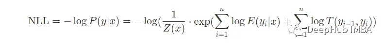
X是输入,y是标签
根据LSTM模型,E(y_i|x)为标签yi在i位置的发射分数,T(y_(i-1), y_i)是CRF的学习转换分数,Z(x)是配分函数,它是一个标准化因子,确保所有可能的标记序列的概率之和为1
对数操作后,它变成:
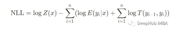
第一项是配分函数的对数,第二项量化LSTM的排放分数与真实标签的匹配程度,而第三项根据CRF说明标签转换的可能性。
由于需要在给定的输入序列中遍历所有可能的标签序列,计算Z(x)的计算量可能会很大:
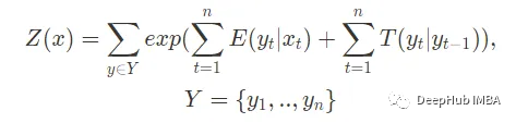
这一过程表现出指数级的时间复杂度。为了解决这个问题,可以使用具有多项式时间复杂度的前向算法。这种方法提供了一种计算配分函数的有效方法,而不需要显式地计算每个可能的标记序列。前向算法依赖于动态规划,特别是利用前向后向算法,该算法在与序列长度线性扩展的时间复杂度下有效地计算配分函数。
配分函数的高效估计
为了理解算法是如何工作的,让我们从一个简单的数值例子开始。现在我们将定义一些玩具发射和转换分数:
 emissions = torch.tensor([    [-0.4554, 0.4215, 0.12],
                               [0.4058, -0.5081, 0.21],
                               [0.2058, 0.5081, 0.02]    ])

 transitions = torch.tensor([ [0.3,  0.1, 0.1],
                              [0.8,  0.2, 0.2],
                              [0.3,  0.7, 0.7] ])
在上一节我们假设每个序列以标记0开始,以标记1结束。通常,它们对应于START_TAG(序列开始标签,又名BOS)和STOP_TAG(序列结束标签,又名EOS),我们通常将STOP_TAG到任何其他标签的转移概率设置为0,将START_TAG从任何其他标签的转移概率设置为1。在这个简单的示例中,我们将忽略这些规则,将允许标记0和1也位于序列的中间。
让我们先来看看如何用一种低效的方法来计算配分函数遍历所有可能的路径
 string_computs = []
 dim_seq_len, dim_lbl = emissions.shape
 scr = 0
 all_s = {}

 for s1 in range(dim_lbl):
     for s2 in range(dim_lbl):
         for s3 in range(dim_lbl):
             # assume sequences start with tag 0 and end with tag 1
             s = (0,) + (s1,)  + (s2,)  + (s3,) + (1,)
             string_computs.append(str(s))
             # note we are in exponential space thus we sum probabilities
             em_sum = 0
             for i in range(len(s)-2):
                 em_sum += emissions[i, s[1:-1][i]].detach().numpy()

             scr_temp = 0
             for i, _ in enumerate(range(len(s)-1)):
                 scr_temp += transitions[s[i], s[i+1]].detach().numpy()

             scr += np.exp(em_sum + scr_temp)
             all_s[s] = em_sum + scr_temp

 print(np.log(scr))
 """
 Output:

 5.0607
 """
当我们手动计算配分函数时,需要循环遍历所有可能的序列,在这种情况下:
 print(string_computs)
 """
 [(0, 0, 0, 0, 1),
  (0, 0, 0, 1, 1),
  (0, 0, 0, 2, 1),
  (0, 0, 1, 0, 1),
  (0, 0, 1, 1, 1),
  (0, 0, 1, 2, 1),
  (0, 0, 2, 0, 1),
  (0, 0, 2, 1, 1),
  (0, 0, 2, 2, 1),
  (0, 1, 0, 0, 1),
  (0, 1, 0, 1, 1),
  (0, 1, 0, 2, 1),
  (0, 1, 1, 0, 1),
  (0, 1, 1, 1, 1),
  (0, 1, 1, 2, 1),
  (0, 1, 2, 0, 1),
  (0, 1, 2, 1, 1),
  (0, 1, 2, 2, 1),
  (0, 2, 0, 0, 1),
  (0, 2, 0, 1, 1),
  (0, 2, 0, 2, 1),
  (0, 2, 1, 0, 1),
  (0, 2, 1, 1, 1),
  (0, 2, 1, 2, 1),
  (0, 2, 2, 0, 1),
  (0, 2, 2, 1, 1),
  (0, 2, 2, 2, 1)]
 """
这不是很有效,因为可以看到多次计算相同的序列,例如(0,0),(0,1),(0,2)计算9次或(0,0,0),(0,0,1),(0,0,2)计算3次等等。所以与其多次重新计算相同的东西,可以计算一次并存储它们以供其他计算:
 START_TAG = 0
 STOP_TAG = 1
 dim_seq_len, dim_lbl = emissions.shape
 init_alphas = transitions[START_TAG] + emissions[START_TAG]

 # Wrap in a variable so that we will get automatic backprop
 alphas = init_alphas
 print(alphas)

 for emission in emissions[1:]:
     alphas_t = []  # The forward tensors at this timestep
     for next_tag in range(dim_lbl):
         # emission score for the next tag
         emit_score = emission[next_tag].view(1, -1).expand(1, dim_lbl)
         # transition score from any previous tag to the next tag
         trans_score = transitions[:, next_tag].view(1, -1)
         # combine current scores with previous alphas
         # since alphas are in log space (see logsumexp below),
         # we add them instead of multiplying
         next_tag_var = alphas + trans_score + emit_score
         print(f"Scores {next_tag} - {next_tag_var} |-| {torch.logsumexp(next_tag_var, dim=1)}")

         alphas_t.append(torch.logsumexp(next_tag_var, 1).view(1))

     alphas = torch.cat(alphas_t).view(1, -1)
     print(alphas)

 terminal_alphas = alphas + transitions[:, STOP_TAG]
 print(terminal_alphas)
 alphas = torch.logsumexp(terminal_alphas, 1)
 print(alphas)

 """
 Outputs:

 tensor([-0.1554,  0.5215,  0.2200])
 Scores 0 - tensor([[0.5504, 1.7273, 0.9258]]) |-| tensor([2.2908])
 Scores 1 - tensor([[-0.5635,  0.2134,  0.4119]]) |-| tensor([1.1990])
 Scores 2 - tensor([[0.1546, 0.9315, 1.1300]]) |-| tensor([1.9171])
 tensor([[2.2908, 1.1990, 1.9171]])
 Scores 0 - tensor([[2.7966, 2.2048, 2.4229]]) |-| tensor([3.6038])
 Scores 1 - tensor([[2.8989, 1.9071, 3.1252]]) |-| tensor([3.8639])
 Scores 2 - tensor([[2.4108, 1.4190, 2.6371]]) |-| tensor([3.3758])
 tensor([[3.6038, 3.8639, 3.3758]])
 tensor([[3.7038, 4.0639, 4.0758]])

 tensor([5.0607])

 """
让我们试着分解它来理解发生了什么:
 alpha0_0 = transitions[START_TAG , 0] + emissions[START_TAG , 0] # (0, 0)
 alpha0_1 = transitions[START_TAG , 1] + emissions[START_TAG , 1] # (0, 1)
 alpha0_2 = transitions[START_TAG , 2] + emissions[START_TAG , 2] # (0, 2)
 print(alpha0_0, alpha0_1, alpha0_2)

 # all combos of len 3 that finish with 0, so (0, 0, 0), (0, 1, 0), (0, 2, 0)
 alpha1_0 = torch.logsumexp(torch.tensor([(eval(f"alpha0_{i}") + transitions[i, 0] + emissions[1, 0]) for i in range(dim_lbl)]).unsqueeze(0), 1)
 # all combos of len 3 that finish with 1, so (0, 0, 1), (0, 1, 1), (0, 2, 1)
 alpha1_1 = torch.logsumexp(torch.tensor([(eval(f"alpha0_{i}") + transitions[i, 1] + emissions[1, 1]) for i in range(dim_lbl)]).unsqueeze(0), 1)
 alpha1_2 = torch.logsumexp(torch.tensor([(eval(f"alpha0_{i}") + transitions[i, 2] + emissions[1, 2]) for i in range(dim_lbl)]).unsqueeze(0), 1)
 print(alpha1_0, alpha1_1, alpha1_2)


 # all combos of len 4 that finish with 0, so (0, 0, 0, 0), (0, 0, 1, 0), (0, 0, 2, 0), .. , (0, 2, 1, 0) , (0, 2, 2, 0)
 alpha2_0 = torch.logsumexp(torch.tensor([(eval(f"alpha1_{i}") + transitions[i, 0] + emissions[2, 0]) for i in range(dim_lbl)]).unsqueeze(0), 1)
 alpha2_1 = torch.logsumexp(torch.tensor([(eval(f"alpha1_{i}") + transitions[i, 1] + emissions[2, 1]) for i in range(dim_lbl)]).unsqueeze(0), 1)
 # all combos of len 4 that finish with 2, so (0, 0, 0, 2), (0, 0, 1, 2), (0, 0, 2, 2), ..,(0, 2, 1, 2) , (0, 2, 2, 2)
 alpha2_2 = torch.logsumexp(torch.tensor([(eval(f"alpha1_{i}") + transitions[i, 2] + emissions[2, 2]) for i in range(dim_lbl)]).unsqueeze(0), 1)
 print(alpha2_0, alpha2_1, alpha2_2)

 alpha3_0 = torch.logsumexp(torch.tensor([(eval(f"alpha2_{i}") + transitions[i, STOP_TAG]) for i in range(dim_lbl)]).unsqueeze(0), 1)
 print(alpha3_0)

 """
 Outputs:

 tensor(-0.1554) tensor(0.5215) tensor(0.2200)
 tensor([2.2908]) tensor([1.1990]) tensor([1.9171])
 tensor([3.6038]) tensor([3.8639]) tensor([3.3758])
 tensor([5.0607])

 """
每个alpha表示具有给定最终标记的所有路径的和。例如,alpha2_0为:
 string_computs = []
 dim_seq_len, dim_lbl = emissions.shape
 scr = 0
 all_s = {}

 # let's recompute all sequences scores first
 for s1 in range(dim_lbl):
     for s2 in range(dim_lbl):
         for s3 in range(dim_lbl):
             s = (START_TAG ,) + (s1,)  + (s2,)  + (s3,)
             string_computs.append(str(s))

             em_sum = 0
             for i in range(len(s)-1):
                 em_sum += emissions[i, s[1:][i]].detach().numpy()

             scr_temp = 0
             for i, _ in enumerate(range(len(s)-1)):
                 scr_temp += transitions[s[i], s[i+1]].detach().numpy()

             scr += np.exp(em_sum + scr_temp)
             all_s[s] = em_sum + scr_temp

 # now let's use `all_s` from above
 cumsum = []
 for e in all_s.keys():
     if e[-1] == 0:
         print(e, all_s[e])
         cumsum.append(all_s[e])

 # sum all probabilities scores
 print(torch.logsumexp(torch.tensor(cumsum).unsqueeze(0), 1))

 """
 Outputs:

 (0, 0, 0, 0) 1.0562000572681427
 (0, 0, 1, 0) 0.44230005890130997
 (0, 0, 2, 0) 0.6604000255465508
 (0, 1, 0, 0) 2.2331000342965126
 (0, 1, 1, 0) 1.219200037419796
 (0, 1, 2, 0) 1.4373000040650368
 (0, 2, 0, 0) 1.431600034236908
 (0, 2, 1, 0) 1.4177000224590302
 (0, 2, 2, 0) 1.635799989104271

 tensor([3.6038], dtype=torch.float64)

 """
这样,假设我们在alpha1_0处到目前为止一直遵循序列(0,0,0)。在这里有3个选择:(0,0,0,0),(0,0,0,1),(0,0,0,2)。而不是重新计算(0,0,0)3次,只计算一次,然后相应添加(0),(1)或(2)。
所以可以将整个过程说明如下:
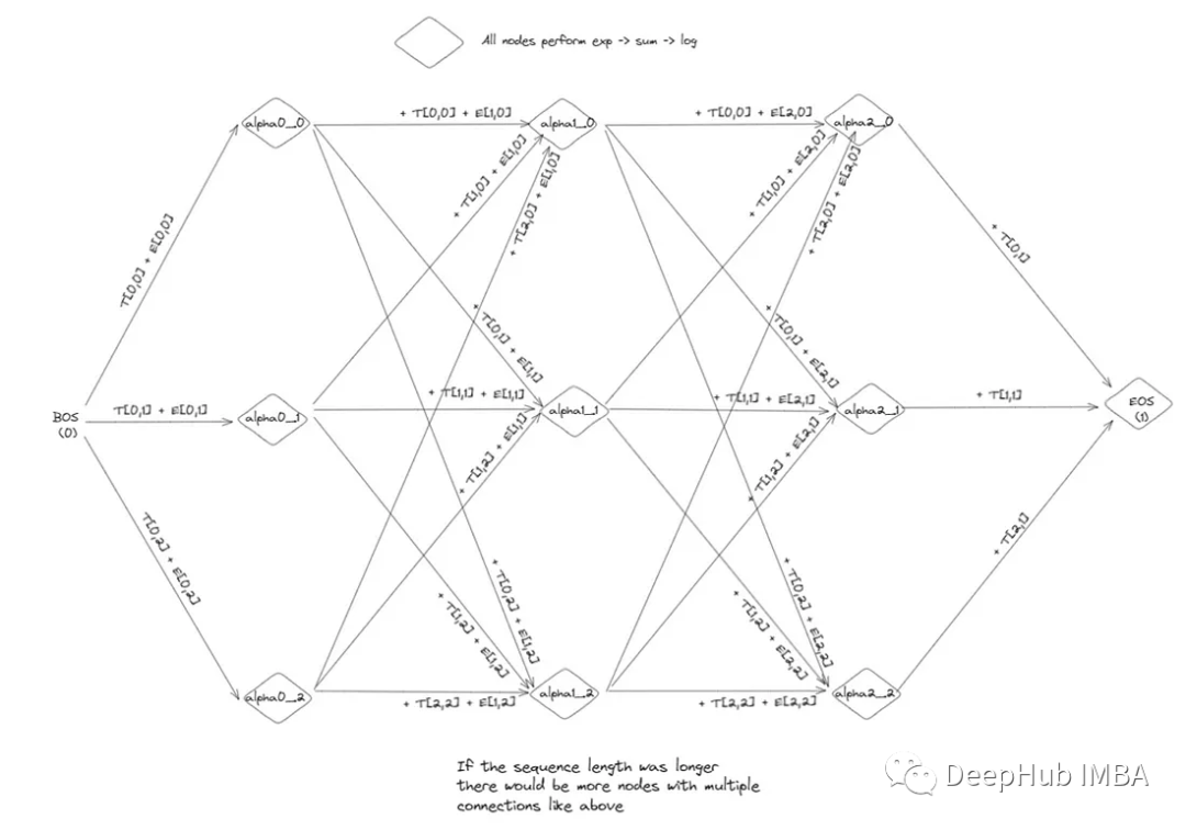
我们已经有效地计算了配分函数Z(x),还需要计算损失的第二部分:
我们的发射和转换分数已经在对数空间中,所以需要以下代码:
 score = torch.zeros(1)
 tags = torch.cat([torch.tensor([START_TAG], dtype=torch.long), tags[0]])
 for i, emission in enumerate(emissions):
     score = score + transitions[tags[i], tags[i+1]] + emission[tags[i+1]]
 score = score + transitions[tags[-1], STOP_TAG]
通过将这两个部分加在一起,可以计算负对数似然损失来训练CRF和LSTM系数。
以上就是计算损失和训练模型的全部过程,那么推理呢?
在推理时,我们需要找到具有最高概率的序列,这与计算配分函数有类似的问题-它具有指数时间,因为我们需要循环遍历所有可能的序列。解决方案是使用另一种类似算法的递归能力,称为Viterbi算法。
Viterbi算法进行推理
根据数据估计的发射和转换分数,需要使用Viterbi算法来选择概率最高的序列(见图1 - CRF层示例)。与前向算法类似,Viterbi算法允许我们有效地估计它,而不是计算所有可能的序列得分并在最后选择得分最高的一个。
 transitions = torch.tensor([  [-1.0000e+04, -9.3,  0.6,  0.1,  0.6],
                               [-1.0000e+04, -1.0000e+04, -1.0000e+04, -1.0000e+04, -1.0000e+04],
                               [-1.0000e+04, -2,  -6,  0.9, 0.1],
                               [-1.0000e+04, 0.2,  -4, -5, 0.3],
                               [-1.0000e+04, 0.5, 0.3, -6.,  0.2]   ]).float()
 transitions = torch.nn.Parameter(transitions)

 emissions = torch.tensor([  [-0.2196,  -1.4047,  0.9992, 0.1948,  0.11],
                             [-0.2401,  0.4565,  0.3464, -0.1856,  0.2622],
                             [-0.3361,  0.1828, -0.3463, -0.2874,  0.2696]   ])
低效的解决方案如下所示,循环遍历所有可能的序列,然后选择得分最高的序列:
 # first recompute scores for all sequences `all_s`
 dim_seq_len, dim_lbl = emissions.shape
 scr = 0
 all_s = {}
 for s1 in range(dim_lbl):
     for s2 in range(dim_lbl):
         for s3 in range(dim_lbl):

             s = (START_TAG ,) + (s1,) + (s2,) + (s3,) + (STOP_TAG,)

             em_sum = 0
             for i in range(len(s)-2):
                 em_sum += emissions[i, s[1:-1][i]].detach().numpy()

             scr_temp = 0
             for i, _ in enumerate(range(len(s)-1)):
                 scr_temp += transitions[s[i], s[i+1]].detach().numpy()

             scr += np.exp(em_sum + scr_temp)
             all_s[s] = em_sum + scr_temp


 sorted(all_s.items(), key=lambda x: x[1])[::-1]

 """
 Most likely sequence is
 (0,2,3,4,1)


 [((0, 2, 3, 4, 1), 3.383200004696846),
  ((0, 2, 4, 4, 1), 2.931000016629696),
  ((0, 4, 2, 4, 1), 2.2260000333189964),
  ((0, 4, 2, 3, 1), 2.1689999997615814),
  ((0, 4, 4, 4, 1), 2.141800031065941),
  ((0, 3, 4, 4, 1), 1.8266000226140022),
  ((0, 2, 4, 2, 1), -0.08489998430013657),
  ((0, 4, 4, 2, 1), -0.8740999698638916),
  ((0, 3, 4, 2, 1), -1.1892999783158302),
  ((0, 3, 2, 4, 1), -2.489199995994568),
  ((0, 3, 2, 3, 1), -2.546200029551983),
  ...
  ((0, 1, 1, 1, 1), -30010.065400242805),
  ((0, 0, 0, 0, 1), -30010.095800206065)]

 """
有效的方法是使用Viterbi算法,如果在计算配分函数Z(X)之前,alpha的范围是找到所有序列的总概率分布,因此alpha是迄今为止序列中所有概率分布的总和,在Viterbi中alpha需要以最高概率遵循序列。所以不是在每个alpha节点上进行求和,而是取最大值,丢弃所有其他路径,就像我们在任何中间阶段选择具有最大alpha的节点一样,因为在给定节点后进行完全相同的计算,所以如果不在该节点上选择最大值,将获得较低的最终分数。
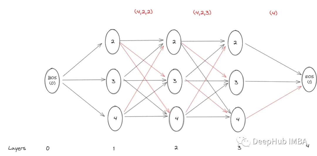
代码将忽略下图中的START_TAG(0)和STOP_TAG(1)节点。
当我们从BOS到下一个节点(第一层)时,我们不能在这个阶段丢弃任何节点,因为具有最大概率的序列可以通过任何节点。
 emission = emission.unsqueeze(0)
 # we only compute these combos once
 # even if in `all_s` below they appear multiple times.
 # Specifically, they appear 9 times each
 alpha0_0 = transitions[START_TAG , 0] + emissions[START_TAG , 0] # (0, 0)
 alpha0_1 = transitions[START_TAG , 1] + emissions[START_TAG , 1] # (0, 1)
 alpha0_2 = transitions[START_TAG , 2] + emissions[START_TAG , 2] # (0, 2)
 alpha0_3 = transitions[START_TAG , 3] + emissions[START_TAG , 3] # (0, 2)
 alpha0_4 = transitions[START_TAG , 4] + emissions[START_TAG , 4] # (0, 2)

 print(alpha0_0, alpha0_1, alpha0_2, alpha0_3,alpha0_4)
 """
 Outputs:

 tensor(-10000.2197, grad_fn=<AddBackward0>)
 tensor(-10.7047, grad_fn=<AddBackward0>)
 tensor(1.5992, grad_fn=<AddBackward0>)
 tensor(0.2948, grad_fn=<AddBackward0>)
 tensor(0.7100, grad_fn=<AddBackward0>)
 """
在第二层情况就不一样了——可以从之前的节点2、3和4转到节点2。在这里只选择导致最大值的路径,因为我们对之后的任何节点都进行了完全相同的计算,如果我们没有在这个节点上选择最大值,最终分数会更低。
 alpha1_0_val, alpha1_0_idx = torch.max(torch.tensor([(eval(f"alpha0_{i}") + transitions[i, 0] + emissions[1, 0]) for i in range(5)]).unsqueeze(0), 1)
 alpha1_1_val, alpha1_1_idx = torch.max(torch.tensor([(eval(f"alpha0_{i}") + transitions[i, 1] + emissions[1, 1]) for i in range(5)]).unsqueeze(0), 1)
 alpha1_2_val, alpha1_2_idx = torch.max(torch.tensor([(eval(f"alpha0_{i}") + transitions[i, 2] + emissions[1, 2]) for i in range(5)]).unsqueeze(0), 1)
 alpha1_3_val, alpha1_3_idx = torch.max(torch.tensor([(eval(f"alpha0_{i}") + transitions[i, 3] + emissions[1, 3]) for i in range(5)]).unsqueeze(0), 1)
 alpha1_4_val, alpha1_4_idx = torch.max(torch.tensor([(eval(f"alpha0_{i}") + transitions[i, 4] + emissions[1, 4]) for i in range(5)]).unsqueeze(0), 1)

 print("*"*100)
 for tag in range(5):
   print(f"Scores to tag {tag}")
     print(torch.tensor([(eval(f"alpha0_{i}") + transitions[i, tag] + emissions[1, tag]) for i in range(5)]).unsqueeze(0))
     print("Max index alpha : ", eval(f"alpha1_{tag}_idx").item())
     print()

 print("Maximum Values:")
 print(alpha1_0_val, alpha1_1_val, alpha1_2_val, alpha1_3_val, alpha1_4_val)
 print("Corresponding Indices:")
 print(alpha1_0_idx, alpha1_1_idx, alpha1_2_idx, alpha1_3_idx, alpha1_4_idx)
 print("*"*100)

 """
 Outputs:

 ****************************************************************************************************
 Scores to tag 0
 tensor([[-20000.4590, -10010.9453,  -9998.6406,  -9999.9453,  -9999.5303]])
 Max index alpha :  2

 Scores to tag 1
 tensor([[-1.0009e+04, -1.0010e+04,  5.5700e-02,  9.5130e-01,  1.6665e+00]])
 Max index alpha :  4

 Scores to tag 2
 tensor([[-9.9993e+03, -1.0010e+04, -4.0544e+00, -3.3588e+00,  1.3564e+00]])
 Max index alpha :  4

 Scores to tag 3
 tensor([[-1.0000e+04, -1.0011e+04,  2.3136e+00, -4.8908e+00, -5.4756e+00]])
 Max index alpha :  2

 Scores to tag 4
 tensor([[-9.9994e+03, -1.0010e+04,  1.9614e+00,  8.5700e-01,  1.1722e+00]])
 Max index alpha :  2

 Maximum Values:
 tensor([-9998.6406]) tensor([1.6665]) tensor([1.3564]) tensor([2.3136]) tensor([1.9614])
 Corresponding Indices:
 tensor([2]) tensor([4]) tensor([4]) tensor([2]) tensor([2])
 ****************************************************************************************************

 """
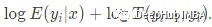
上面的计算告诉我们,如果想要在第2层转换到标签3(标签3的分数),那么最好的标签是从前一层的标签2开始,因为它最终会导致最大的最终分数。如果我们想在第2层转换到标签2(分数到标签2),最好的标签是从标签4开始,以此类推。
图中也说明了这一点-转换到第2层的标签2需要选择第1层的标签4,选择第3层的标签2,选择第4层的标签2。这就是从第1层到第2层的红线以及第1层和第2层之间的元组(4,2,2)所代表的内容。
可以在下面验证:
 layer = 2
 tag = 3
 selected = {}
 for k, v in all_s.items():
     if k[layer] == tag:
         # print(k, v)
         selected[k] = v

 # if we want to transition at layer 2 to tag 3,
 # the best tag to do it is from tag 2
 sorted(selected.items(), key=lambda x: x[1])[::-1][0]
 # ((0, 2, 3, 4, 1), 3.383200004696846) - (tags, path score)

 layer = 2
 tag = 2
 selected = {}
 for k, v in all_s.items():
     if k[layer] == tag:
         # print(k, v)
         selected[k] = v

 # if we want to transition at layer 2 to tag 2,
 # the best tag to do it is from tag 4
 sorted(selected.items(), key=lambda x: x[1])[::-1][0]
 # ((0, 4, 2, 4, 1), 2.2260000333189964) - (tags, path score)
然后是第三层:
 alpha2_0_val, alpha2_0_idx = torch.max(torch.tensor([(eval(f"alpha1_{i}_val") + transitions[i, 0] + emissions[2, 0]) for i in range(5)]).unsqueeze(0), 1)
 alpha2_1_val, alpha2_1_idx = torch.max(torch.tensor([(eval(f"alpha1_{i}_val") + transitions[i, 1] + emissions[2, 1]) for i in range(5)]).unsqueeze(0), 1)
 alpha2_2_val, alpha2_2_idx = torch.max(torch.tensor([(eval(f"alpha1_{i}_val") + transitions[i, 2] + emissions[2, 2]) for i in range(5)]).unsqueeze(0), 1)
 alpha2_3_val, alpha2_3_idx = torch.max(torch.tensor([(eval(f"alpha1_{i}_val") + transitions[i, 3] + emissions[2, 3]) for i in range(5)]).unsqueeze(0), 1)
 alpha2_4_val, alpha2_4_idx = torch.max(torch.tensor([(eval(f"alpha1_{i}_val") + transitions[i, 4] + emissions[2, 4]) for i in range(5)]).unsqueeze(0), 1)

 print("*"*100)
 for tag in range(5):
     print(f"Scores for tag {tag}")
     print(torch.tensor([(eval(f"alpha1_{i}_val") + transitions[i, tag] + emissions[2, tag]) for i in range(5)]).unsqueeze(0))
     print("Max index alpha : ", eval(f"alpha2_{tag}_idx").item())
     print()

 print(alpha2_0_val, alpha2_1_val, alpha2_2_val, alpha2_3_val, alpha2_4_val)
 print(alpha2_0_idx, alpha2_1_idx, alpha2_2_idx, alpha2_3_idx, alpha2_4_idx)
 print("*"*100)


 """
 Outputs:

 ****************************************************************************************************
 Scores to tag 0
 tensor([[-19998.9766,  -9998.6699,  -9998.9795,  -9998.0225,  -9998.3750]])
 Max index alpha :  3

 Scores to tag 1
 tensor([[-1.0008e+04, -9.9982e+03, -4.6080e-01,  2.6964e+00,  2.6442e+00]])
 Max index alpha :  3

 Scores to tag 2
 tensor([[-9.9984e+03, -9.9987e+03, -4.9899e+00, -2.0327e+00,  1.9151e+00]])
 Max index alpha :  4

 Scores to tag 3
 tensor([[-9.9988e+03, -9.9986e+03,  1.9690e+00, -2.9738e+00, -4.3260e+00]])
 Max index alpha :  2

 Scores to tag 4
 tensor([[-9.9978e+03, -9.9981e+03,  1.7260e+00,  2.8832e+00,  2.4310e+00]])
 Max index alpha :  3

 Maximum Values:
 tensor([-9998.0225]) tensor([2.6964]) tensor([1.9151]) tensor([1.9690]) tensor([2.8832])
 Corresponding Indices:
 tensor([3]) tensor([3]) tensor([4]) tensor([2]) tensor([3])
 ****************************************************************************************************
 """
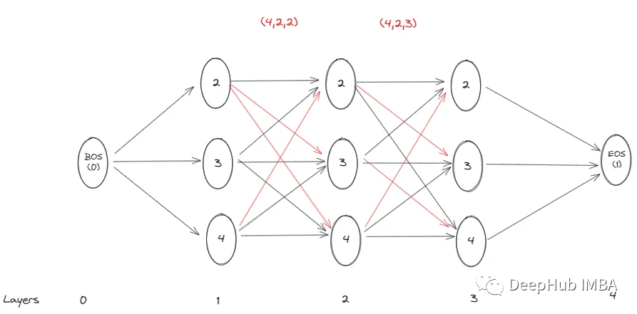
在最后的第4层是我们的递归停止的地方,可以选择最大序列的最后一个节点(在STOP_TAG之前),然后从那里回溯到找到整个最大序列
 alpha3_0_val, alpha3_0_idx = torch.max(torch.tensor([(eval(f"alpha2_{i}_val") + transitions[i, 1]) for i in range(5)]).unsqueeze(0), 1)
 print(torch.tensor([(eval(f"alpha2_{i}_val") + transitions[i, 1]) for i in range(5)]).unsqueeze(0))
 print(alpha3_0_val, alpha3_0_idx)
 """
 tensor([[-1.0007e+04, -9.9973e+03, -8.4900e-02,  2.1690e+00,  3.3832e+00]])
 tensor([3.3832]) tensor([4])
 """
把上面所有的代码进行整合后:
 dim_seq_len, dim_lbl = emissions.shape

 backpointers = []
 # Initialize the viterbi variables in log space
 init_alphas = transitions[START_TAG ] + emissions[:1]

 # alphas at step i holds the viterbi variables for step i-1
 alphas = init_alphas
 print("*" * 100)
 print("Start Alphas : ", alphas)
 print("*" * 100)
 for l, emission in enumerate(emissions[1:], 1):
     bptrs_t = []  # holds the backpointers for this step
     viterbivars_t = []  # holds the viterbi variables for this step

     for next_tag in range(crf_mod.num_tags):
         # next_tag_var[i] holds the viterbi variable for tag i at the
         # previous step, plus the score of transitioning
         # from tag i to next_tag.
         # We don't include the emission scores here because the max
         # does not depend on them (we add them in below)
         next_tag_var = alphas + transitions[:, next_tag] + emission[next_tag]
         best_tag_score, best_tag_id = torch.max(next_tag_var, dim=-1)
         bptrs_t.append(best_tag_id)
         viterbivars_t.append(next_tag_var[0][best_tag_id].view(1))
         print(f"Scores for tag {next_tag} - {next_tag_var}\n Max index alpha : {best_tag_id.item()}, max value alpha : {best_tag_score.item()}")

     # Now add in the emission scores, and assign alphas to the set
     # of viterbi variables we just computed
     alphas = (torch.cat(viterbivars_t)).view(1, -1)
     print("*" * 100)
     print(f"Alphas layer {l}: ", alphas)
     print("*" * 100)
     backpointers.append(bptrs_t)

 # Transition to STOP_TAG
 terminal_alphas = alphas + transitions[:, STOP_TAG]
 # best tag at the end of the sequence (before the STOP_TAG)
 best_tag_score, best_tag_id = torch.max(terminal_alphas, dim=-1)
 print("*" * 100)
 print("End Alphas : ", terminal_alphas)
 print("*" * 100)

 print(f"Max index alpha : {best_tag_id.item()}, max value alpha : {best_tag_score.item()}")


 """
 Outputs:

 ****************************************************************************************************
 Start Alphas :  tensor([[-1.0000e+04, -1.0705e+01,  1.5992e+00,  2.9480e-01,  7.1000e-01]],
        grad_fn=<AddBackward0>)
 ****************************************************************************************************
 Scores for tag 0 - tensor([[-20000.4590, -10010.9453,  -9998.6406,  -9999.9453,  -9999.5303]],
        grad_fn=<AddBackward0>)
  Max index alpha : 2, max value alpha : -9998.640625
 Scores for tag 1 - tensor([[-1.0009e+04, -1.0010e+04,  5.5700e-02,  9.5130e-01,  1.6665e+00]],
        grad_fn=<AddBackward0>)
  Max index alpha : 4, max value alpha : 1.6665000915527344
 Scores for tag 2 - tensor([[-9.9993e+03, -1.0010e+04, -4.0544e+00, -3.3588e+00,  1.3564e+00]],
        grad_fn=<AddBackward0>)
  Max index alpha : 4, max value alpha : 1.3564000129699707
 Scores for tag 3 - tensor([[-1.0000e+04, -1.0011e+04,  2.3136e+00, -4.8908e+00, -5.4756e+00]],
        grad_fn=<AddBackward0>)
  Max index alpha : 2, max value alpha : 2.3135998249053955
 Scores for tag 4 - tensor([[-9.9994e+03, -1.0010e+04,  1.9614e+00,  8.5700e-01,  1.1722e+00]],
        grad_fn=<AddBackward0>)
  Max index alpha : 2, max value alpha : 1.961400032043457
 ****************************************************************************************************
 Alphas layer 1:  tensor([[-9.9986e+03,  1.6665e+00,  1.3564e+00,  2.3136e+00,  1.9614e+00]],
        grad_fn=<ViewBackward>)
 ****************************************************************************************************
 Scores for tag 0 - tensor([[-19998.9766,  -9998.6699,  -9998.9795,  -9998.0225,  -9998.3750]],
        grad_fn=<AddBackward0>)
  Max index alpha : 3, max value alpha : -9998.0224609375
 Scores for tag 1 - tensor([[-1.0008e+04, -9.9982e+03, -4.6080e-01,  2.6964e+00,  2.6442e+00]],
        grad_fn=<AddBackward0>)
  Max index alpha : 3, max value alpha : 2.6963999271392822
 Scores for tag 2 - tensor([[-9.9984e+03, -9.9987e+03, -4.9899e+00, -2.0327e+00,  1.9151e+00]],
        grad_fn=<AddBackward0>)
  Max index alpha : 4, max value alpha : 1.9150999784469604
 Scores for tag 3 - tensor([[-9.9988e+03, -9.9986e+03,  1.9690e+00, -2.9738e+00, -4.3260e+00]],
        grad_fn=<AddBackward0>)
  Max index alpha : 2, max value alpha : 1.9690001010894775
 Scores for tag 4 - tensor([[-9.9978e+03, -9.9981e+03,  1.7260e+00,  2.8832e+00,  2.4310e+00]],
        grad_fn=<AddBackward0>)
  Max index alpha : 3, max value alpha : 2.883199691772461
 ****************************************************************************************************
 Alphas layer 2:  tensor([[-9.9980e+03,  2.6964e+00,  1.9151e+00,  1.9690e+00,  2.8832e+00]],
        grad_fn=<ViewBackward>)
 ****************************************************************************************************
 ****************************************************************************************************
 End Alphas :  tensor([[-1.0007e+04, -9.9973e+03, -8.4900e-02,  2.1690e+00,  3.3832e+00]],
        grad_fn=<AddBackward0>)
 ****************************************************************************************************
 Max index alpha : 4, max value alpha : 3.383199691772461

 """
可以为我们的句子找到最可能的标签序列:
 # get the final most probable score and the final most probable tag
 # (tag 4 in the illustration)
 best_path = [best_tag_id]

 # Follow the back pointers to decode the best path.
 for bptrs_t in reversed(backpointers):
   # best tag to follow given best tag from next layer
     best_tag_id = bptrs_t[best_tag_id]
     best_path.append(best_tag_id)

 # reverse best path list
 best_path.reverse()
 best_path = torch.cat(best_path)

 path_score, best_path


 """
 Outputs:

 (tensor([3.3832], grad_fn=<IndexBackward>), tensor([2, 3, 4]))

 """
以上图为例,我们做个更详细的流程描述:
首先在第三层找到alpha分数最大的标签 4。现在使用之前发现的最大alpha来找到需要从第2层选择的标签,因为第3层的标签是4 -第2层为 3。然后对前一层做同样的事情得到 2。因此根据Viterbi算法,具有最高概率得分的序列是(0,2,3,4,1),这与我们使用低效解决方案更快地找到的结果相同,因为我们在每个中间alpha节点上丢弃了除1条路径外的所有路径。
完整的LSTM-CRF代码
 import torch
 import torch.nn as nn

 IMPOSSIBLE = -1e4

 class BiLSTM_CRF(nn.Module):

     def __init__(
         self, vocab_size, num_tags, start_tag, stop_tag,
         embedding_dim, hidden_dim
     ):
         super().__init__()

         self.num_tags = num_tags
         self.START_TAG = start_tag
         self.STOP_TAG = stop_tag

         # CRF parameters
         self.transitions = nn.Parameter(torch.randn(self.num_tags, self.num_tags))

         # These two statements enforce the constraint that we never transfer
         # to the start tag and we never transfer from the stop tag
         self.transitions.data[:, self.START_TAG] = IMPOSSIBLE
         self.transitions.data[self.STOP_TAG, :] = IMPOSSIBLE

         # LSTM parameters
         self.hidden_dim = hidden_dim
         self.word_embeds = nn.Embedding(vocab_size, embedding_dim)
         self.lstm = nn.LSTM(embedding_dim, hidden_dim // 2,
                             num_layers=1, bidirectional=True,
                             batch_first=False)

         # Maps the output of the LSTM into tag space.
         self.hidden2tag = nn.Linear(hidden_dim, self.num_tags)

         self.hidden = self.init_hidden()

     def init_hidden(self):
         return (torch.randn(2, 1, self.hidden_dim // 2),
                 torch.randn(2, 1, self.hidden_dim // 2))

     def _get_emissions(self, sentence):
         self.hidden = self.init_hidden()
         embeds = self.word_embeds(sentence).view(len(sentence), 1, -1)
         lstm_out, self.hidden = self.lstm(embeds, self.hidden)
         lstm_out = lstm_out.view(len(sentence), self.hidden_dim)
         emissions = self.hidden2tag(lstm_out)
         return emissions

     def neg_log_likelihood(self, sentence, tags):
         emissions = self._get_emissions(sentence)
         forward_score = self._forward_alg(emissions)
         gold_score = self._score_sentence(emissions, tags)
         return forward_score - gold_score

     def _forward_alg(self, emissions):

         init_alphas = self.transitions[self.START_TAG] + emissions[0]

         # Wrap in a variable so that we will get automatic backprop
         alphas = init_alphas

         for emission in emissions[1:]:
             alphas_t = []  # The forward tensors at this timestep
             for next_tag in range(self.num_tags):
                 # emission score for the next tag
                 emit_score = emission[next_tag].view(1, -1).expand(1, self.num_tags)
                 # transition score from any previous tag to the next tag
                 trans_score = self.transitions[:, next_tag].view(1, -1)
                 # combine current scores with previous alphas
                 # since alphas are in log space (see logsumexp below),
                 # we add them instead of multiplying
                 next_tag_var = alphas + trans_score + emit_score

                 alphas_t.append(torch.logsumexp(next_tag_var, 1).view(1))

             alphas = torch.cat(alphas_t).view(1, -1)

         terminal_alphas = alphas + self.transitions[:, self.STOP_TAG]
         alphas = torch.logsumexp(terminal_alphas, 1)

         return alphas

     def _viterbi_decode(self, emissions):
         backpointers = []

         # Initialize the viterbi variables in log space
         init_alphas = self.transitions[self.START_TAG] + emissions[:1]

         # alphas at step i holds the viterbi variables for step i-1
         alphas = init_alphas
         for emission in emissions[1:]:
             bptrs_t = []  # holds the backpointers for this step
             viterbivars_t = []  # holds the viterbi variables for this step

             for next_tag in range(self.num_tags):
                 # next_tag_var[i] holds the viterbi variable for tag i at the
                 # previous step, plus the score of transitioning
                 # from tag i to next_tag.
                 # We don't include the emission scores here because the max
                 # does not depend on them (we add them in below)
                 next_tag_var = alphas + self.transitions[:, next_tag] + emission[next_tag]
                 best_tag_score, best_tag_id = torch.max(next_tag_var, dim=-1)
                 bptrs_t.append(best_tag_id)
                 viterbivars_t.append(next_tag_var[0][best_tag_id].view(1))
             # Now add in the emission scores, and assign alphas to the set
             # of viterbi variables we just computed
             alphas = (torch.cat(viterbivars_t)).view(1, -1)
             backpointers.append(bptrs_t)

         # Transition to STOP_TAG
         terminal_alphas = alphas + self.transitions[:, self.STOP_TAG]
         best_tag_score, best_tag_id = torch.max(terminal_alphas, dim=-1)
         path_score = terminal_alphas[0][best_tag_id]

         # Follow the back pointers to decode the best path.
         # Append terminal tag
         best_path = [best_tag_id]
         for bptrs_t in reversed(backpointers):
             best_tag_id = bptrs_t[best_tag_id]
             best_path.append(best_tag_id)

         best_path.reverse()
         best_path = torch.cat(best_path)

         return path_score, best_path

     def forward(self, sentence):
         # Get the emission scores from the BiLSTM
         emissions = self._get_emissions(sentence)
         print(emissions)

         # Find the best path, given the emission scores.
         score, tag_seq = self._viterbi_decode(emissions)
         return score, tag_seq

     def _score_sentence(self, emissions, tags):
         # Gives the score of a provided tag sequence
         score = torch.zeros(1)
         tags = torch.cat([torch.tensor([self.START_TAG], dtype=torch.long), tags[0]])
         for i, emission in enumerate(emissions):
             score = score + self.transitions[tags[i], tags[i+1]] + emission[tags[i+1]]
         score = score + self.transitions[tags[-1], self.STOP_TAG]
         return score

 def prepare_sequence(seq, to_ix):
     idxs = [to_ix[w] for w in seq]
     return torch.tensor(idxs, dtype=torch.long)


 if __name__ == '__main__':

     START_TAG = "<START>"
     STOP_TAG = "<STOP>"
     EMBEDDING_DIM = 5
     HIDDEN_DIM = 4

     training_data = [
         (
             "Google Deepmind company".split(),
             "B I O".split(),
         )
     ]


     word_to_ix = {START_TAG: 0, STOP_TAG: 1}
     for sentence, tags in training_data:
         for word in sentence:
             if word not in word_to_ix:
                 word_to_ix[word] = len(word_to_ix)

     tag_to_ix = {START_TAG: 0, STOP_TAG: 1, 'B': 2, 'I': 3, 'O': 4}
     print(word_to_ix)

     crf_mod = BiLSTM_CRF(len(word_to_ix), len(tag_to_ix), tag_to_ix[START_TAG], tag_to_ix[STOP_TAG],
                           embedding_dim=EMBEDDING_DIM, hidden_dim=HIDDEN_DIM)


     sentence, tags = training_data[0]
     sentence_in = prepare_sequence(sentence, word_to_ix)
     targets = torch.tensor([tag_to_ix[t] for t in tags], dtype=torch.long)


     torch.manual_seed(1)
     print(sentence_in, targets)

     score, tag_seq = crf_mod(sentence_in)
     print(score, tag_seq)
CRFs的缺点和总结
在过去,CRF-LSTM模型已被广泛用于序列标记任务,但与最近的Transformer模型相比,它们也存在一定的缺点。一个重要的缺点是,CRF-LSTM不擅长对序列元素之间的长期依赖关系进行建模,而倾向于更好地处理局部上下文。这与transformer的情况不同,因为它们的自注意力机制能够捕获远程依赖关系,擅长建模全局上下文
CRF-LSTM模型的另一个问题是它们顺序处理序列,这限制了并行化,并且对于长序列可能很慢,而transformer并行处理序列,因此通常更快。
但是CRF-LSTM模型的一个重要优点是它的可解释性,因为我们可以探索和理解转换和发射矩阵,而解释Transformer模型则更加困难。
作者:Alexey Kravets