
2017年推出《Attention is All You Need》以来,transformers 已经成为自然语言处理(NLP)的最新技术。2021年,《An Image is Worth 16x16 Words》,成功地将transformers 用于计算机视觉任务。从那时起,许多基于transformers的计算机视觉体系结构被提出。
本文将深入探讨注意力层在计算机视觉环境中的工作原理。我们将讨论单头注意力和多头注意力。它包括注意力层的代码,以及基础数学的概念解释。
在NLP应用中,注意力通常被描述为句子中单词(标记)之间的关系。而在计算机视觉应用程序中,注意力关注图像中patches (标记)之间的关系。
有多种方法可以将图像分解为一系列标记。原始的ViT²将图像分割成小块,然后将小块平摊成标记。《token -to- token ViT》³开发了一种更复杂的从图像创建标记的方法。
点积注意力
《Attention is All You Need》中定义的点积(相当于乘法)注意力是目前我们最常见也是最简单的一种中注意力机制,他的代码实现非常简单:
classAttention(nn.Module):
def__init__(self,
dim: int,
chan: int,
num_heads: int=1,
qkv_bias: bool=False,
qk_scale: NoneFloat=None):
""" Attention Module
Args:
dim (int): input size of a single token
chan (int): resulting size of a single token (channels)
num_heads(int): number of attention heads in MSA
qkv_bias (bool): determines if the qkv layer learns an addative bias
qk_scale (NoneFloat): value to scale the queries and keys by;
if None, queries and keys are scaled by ``head_dim ** -0.5``
"""
super().__init__()
## Define Constants
self.num_heads=num_heads
self.chan=chan
self.head_dim=self.chan//self.num_heads
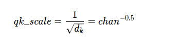
self.scale=qk_scaleorself.head_dim**-0.5
assertself.chan%self.num_heads==0, '"Chan" must be evenly divisible by "num_heads".'
## Define Layers
self.qkv=nn.Linear(dim, chan*3, bias=qkv_bias)
#### Each token gets projected from starting length (dim) to channel length (chan) 3 times (for each Q, K, V)
self.proj=nn.Linear(chan, chan)
defforward(self, x):
B, N, C=x.shape
## Dimensions: (batch, num_tokens, token_len)
## Calcuate QKVs
qkv=self.qkv(x).reshape(B, N, 3, self.num_heads, self.head_dim).permute(2, 0, 3, 1, 4)
#### Dimensions: (3, batch, heads, num_tokens, chan/num_heads = head_dim)
q, k, v=qkv[0], qkv[1], qkv[2]
## Calculate Attention
attn= (q*self.scale) @k.transpose(-2, -1)
attn=attn.softmax(dim=-1)
#### Dimensions: (batch, heads, num_tokens, num_tokens)
## Attention Layer
x= (attn@v).transpose(1, 2).reshape(B, N, self.chan)
#### Dimensions: (batch, heads, num_tokens, chan)
## Projection Layers
x=self.proj(x)
## Skip Connection Layer
v=v.transpose(1, 2).reshape(B, N, self.chan)
x=v+x
#### Because the original x has different size with current x, use v to do skip connection
returnx
单头注意力
对于单个注意力头,让我们逐步了解向前传递每一个patch,使用7 * 7=49作为起始patch大小(因为这是T2T-ViT模型中的起始标记大小)。通道数64这也是T2T-ViT的默认值。然后假设有100标记,并且使用批大小为13进行前向传播(选择这两个数值是为了不会与任何其他参数混淆)。
 # Define an Input
 token_len=7*7
 channels=64
 num_tokens=100
 batch=13
 x=torch.rand(batch, num_tokens, token_len)
 B, N, C=x.shape
 print('Input dimensions are\n\tbatchsize:', x.shape[0], '\n\tnumber of tokens:', x.shape[1], '\n\ttoken size:', x.shape[2])

 # Define the Module
 A=Attention(dim=token_len, chan=channels, num_heads=1, qkv_bias=False, qk_scale=None)
 A.eval();
输入的维度是这样的额:
 Input dimensions are
    batchsize: 13
    number of tokens: 100
    token size: 49
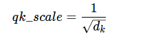
根据查询、键和值矩阵定义的。第一步是通过一个可学习的线性层来计算这些。qkv_bias项表示这些线性层是否有偏置项。这一步还将标记的长度从输入49更改为chan参数(64)。
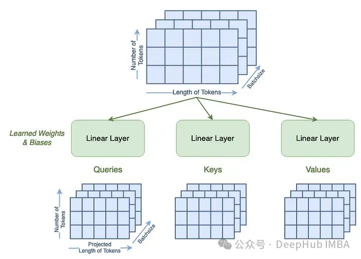
 qkv=A.qkv(x).reshape(B, N, 3, A.num_heads, A.head_dim).permute(2, 0, 3, 1, 4)
 q, k, v=qkv[0], qkv[1], qkv[2]
 print('Dimensions for Queries are\n\tbatchsize:', q.shape[0], '\n\tattention heads:', q.shape[1], '\n\tnumber of tokens:', q.shape[2], '\n\tnew length of tokens:', q.shape[3])
 print('See that the dimensions for queries, keys, and values are all the same:')
 print('\tShape of Q:', q.shape, '\n\tShape of K:', k.shape, '\n\tShape of V:', v.shape)
可以看到 查询、键和值的维度是相同的,13代表批次,1是我们的注意力头数,100是我们输入的标记长度(序列长度),64是我们的通道数。
 Dimensions for Queries are
    batchsize: 13
    attention heads: 1
    number of tokens: 100
    new length of tokens: 64
 See that the dimensions for queries, keys, and values are all the same:
    Shape of Q: torch.Size([13, 1, 100, 64])
    Shape of K: torch.Size([13, 1, 100, 64])
    Shape of V: torch.Size([13, 1, 100, 64])
我们看看可注意力是如何计算的,它被定义为:
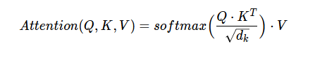
Q、K、V分别为查询、键和值;dₖ是键的维数,它等于键标记的长度,也等于键的长度。
第一步是计算:
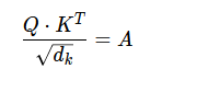
然后是
最后
Q·K的矩阵乘法看起来是这样的
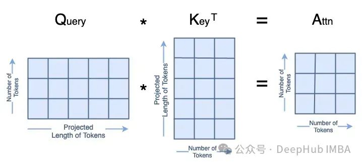
这些就是我们注意力的主要部分,代码是这样的
 attn= (q*A.scale) @k.transpose(-2, -1)
 print('Dimensions for Attn are\n\tbatchsize:', attn.shape[0], '\n\tattention heads:', attn.shape[1], '\n\tnumber of tokens:', attn.shape[2], '\n\tnumber of tokens:', attn.shape[3])
结果如下:
 Dimensions for Attn are
    batchsize: 13
    attention heads: 1
    number of tokens: 100
    number of tokens: 100
下一步就是计算A的softmax,这不会改变它的形状。
attn=attn.softmax(dim=-1)
最后,我们计算出A·V=x:
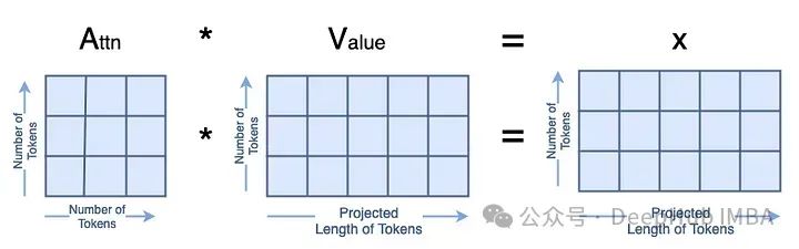
 x=attn@v
 print('Dimensions for x are\n\tbatchsize:', x.shape[0], '\n\tattention heads:', x.shape[1], '\n\tnumber of tokens:', x.shape[2], '\n\tlength of tokens:', x.shape[3])
就得到了我们最终的结果
 Dimensions for x are
    batchsize: 13
    attention heads: 1
    number of tokens: 100
    length of tokens: 64
因为只有一个头,所以我们去掉头数 1
x = x.transpose(1, 2).reshape(B, N, A.chan)
然后我们将x输入一个可学习的线性层,这个线性层不会改变它的形状。
x=A.proj(x)
最后我们实现的跳过连接
 orig_shape= (batch, num_tokens, token_len)
 curr_shape= (x.shape[0], x.shape[1], x.shape[2])
 v=v.transpose(1, 2).reshape(B, N, A.chan)
 v_shape= (v.shape[0], v.shape[1], v.shape[2])
 print('Original shape of input x:', orig_shape)
 print('Current shape of x:', curr_shape)
 print('Shape of V:', v_shape)
 x=v+x
 print('After skip connection, dimensions for x are\n\tbatchsize:', x.shape[0], '\n\tnumber of tokens:', x.shape[1], '\n\tlength of tokens:', x.shape[2])
结果如下:
 Original shape of input x: (13, 100, 49)
 Current shape of x: (13, 100, 64)
 Shape of V: (13, 100, 64)
 After skip connection, dimensions for x are
    batchsize: 13
    number of tokens: 100
    length of tokens: 64
这是我们单头注意力层!
多头注意力
我们可以扩展到多头注意。在计算机视觉中,这通常被称为多头自注意力(MSA)。我们不会详细介绍所有步骤,而是关注矩阵形状不同的地方。
对于多头的注意力,注意力头的数量必须可以整除以通道的数量,所以在这个例子中,我们将使用4个注意头。
 # Define an Input
 token_len=7*7
 channels=64
 num_tokens=100
 batch=13
 num_heads=4
 x=torch.rand(batch, num_tokens, token_len)
 B, N, C=x.shape
 print('Input dimensions are\n\tbatchsize:', x.shape[0], '\n\tnumber of tokens:', x.shape[1], '\n\ttoken size:', x.shape[2])

 # Define the Module
 MSA=Attention(dim=token_len, chan=channels, num_heads=num_heads, qkv_bias=False, qk_scale=None)
 MSA.eval();
结果如下:
 Input dimensions are
    batchsize: 13
    number of tokens: 100
    token size: 49
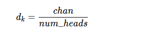
计算查询、键和值的过程与单头的过程相同。但是可以看到标记的新长度是chan/num_heads。Q、K和V矩阵的总大小没有改变;它们的内容只是分布在头部维度上。你可以把它看作是将单个矩阵分割为多个:

我们将子矩阵表示为Qₕ对于查询头i。
 qkv=MSA.qkv(x).reshape(B, N, 3, MSA.num_heads, MSA.head_dim).permute(2, 0, 3, 1, 4)
 q, k, v=qkv[0], qkv[1], qkv[2]
 print('Head Dimension = chan / num_heads =', MSA.chan, '/', MSA.num_heads, '=', MSA.head_dim)
 print('Dimensions for Queries are\n\tbatchsize:', q.shape[0], '\n\tattention heads:', q.shape[1], '\n\tnumber of tokens:', q.shape[2], '\n\tnew length of tokens:', q.shape[3])
 print('See that the dimensions for queries, keys, and values are all the same:')
 print('\tShape of Q:', q.shape, '\n\tShape of K:', k.shape, '\n\tShape of V:', v.shape)
输出如下:
 Head Dimension = chan / num_heads = 64 / 4 = 16
 Dimensions for Queries are
    batchsize: 13
    attention heads: 4
    number of tokens: 100
    new length of tokens: 16
 See that the dimensions for queries, keys, and values are all the same:
    Shape of Q: torch.Size([13, 4, 100, 16])
    Shape of K: torch.Size([13, 4, 100, 16])
    Shape of V: torch.Size([13, 4, 100, 16])
这里需要注意的是
我们需要除以头数。num_heads = 4个不同的Attn矩阵,看起来像:
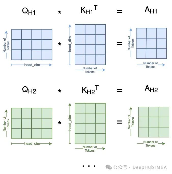
 attn= (q*MSA.scale) @k.transpose(-2, -1)
 print('Dimensions for Attn are\n\tbatchsize:', attn.shape[0], '\n\tattention heads:', attn.shape[1], '\n\tnumber of tokens:', attn.shape[2], '\n\tnumber of tokens:', attn.shape[3]
维度:
 Dimensions for Attn are
    batchsize: 13
    attention heads: 4
    number of tokens: 100
    number of tokens: 100
softmax 不会改变维度,我们略过,然后计算每一个头
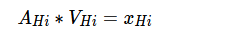
这在多个注意头中是这样的: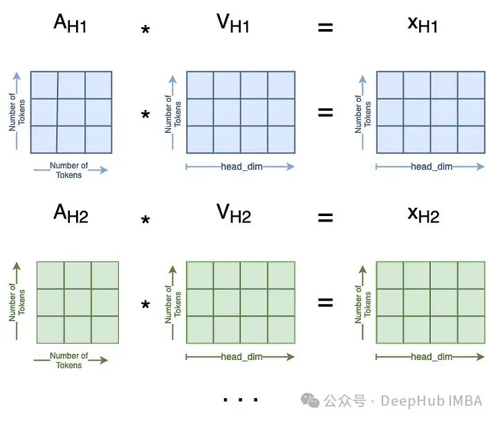
 attn = attn.softmax(dim=-1)

 x = attn @ v
 print('Dimensions for x are\n\tbatchsize:', x.shape[0], '\n\tattention heads:', x.shape[1], '\n\tnumber of tokens:', x.shape[2], '\n\tlength of tokens:', x.shape[3]
维度如下:
 Dimensions for x are
    batchsize: 13
    attention heads: 4
    number of tokens: 100
    length of tokens: 16
最后需要维度重塑并把把所有的xₕ` s连接在一起。这是第一步的逆操作:
 x=x.transpose(1, 2).reshape(B, N, MSA.chan)
 print('Dimensions for x are\n\tbatchsize:', x.shape[0], '\n\tnumber of tokens:', x.shape[1], '\n\tlength of tokens:', x.shape[2])
结果如下:
 Dimensions for x are
    batchsize: 13
    number of tokens: 100
    length of tokens: 64
我们已经将所有头的输出连接在一起,注意力模块的其余部分保持不变。
 x = MSA.proj(x)
 print('Dimensions for x are\n\tbatchsize:', x.shape[0], '\n\tnumber of tokens:', x.shape[1], '\n\tlength of tokens:', x.shape[2])

 orig_shape = (batch, num_tokens, token_len)
 curr_shape = (x.shape[0], x.shape[1], x.shape[2])
 v = v.transpose(1, 2).reshape(B, N, A.chan)
 v_shape = (v.shape[0], v.shape[1], v.shape[2])
 print('Original shape of input x:', orig_shape)
 print('Current shape of x:', curr_shape)
 print('Shape of V:', v_shape)
 x = v + x
 print('After skip connection, dimensions for x are\n\tbatchsize:', x.shape[0], '\n\tnumber of tokens:', x.shape[1], '\n\tlength of tokens:', x.shape[2])
结果如下:
 Dimensions for x are
    batchsize: 13
    number of tokens: 100
    length of tokens: 64
 Original shape of input x: (13, 100, 49)
 Current shape of x: (13, 100, 64)
 Shape of V: (13, 100, 64)
 After skip connection, dimensions for x are
    batchsize: 13
    number of tokens: 100
    length of tokens: 64
这就是多头注意力!
总结
在这篇文章中我们完成了ViT中注意力层。为了更详细的说明我们进行了手动的代码编写,如果要实际的应用,可以使用PyTorch中的torch.nn. multiheadeattention(),因为他的实现要快的多。
最后参考文章:
[1] Vaswani et al (2017). *Attention Is All You Need.*https://doi.org/10.48550/arXiv.1706.03762
[2] Dosovitskiy et al (2020). *An Image is Worth 16x16 Words: Transformers for Image Recognition at Scale.*https://doi.org/10.48550/arXiv.2010.11929
[3] Yuan et al (2021). Tokens-to-Token ViT: Training Vision Transformers from Scratch on ImageNet. https://doi.org/10.48550/arXiv.2101.11986GitHub code: https://github.com/yitu-opensource/T2T-ViT
作者:Skylar Jean Callis